
DMSP/OLS夜间灯光影像中国区域的校正及应用
作者简介:曹子阳(1988-),男,博士生,研究方向为区域可持续发展与城市遥感。E-mail: eationcao@163.com
收稿日期: 2014-12-08
要求修回日期: 2015-01-04
网络出版日期: 2015-09-07
基金资助
国家自然科学基金项目“环珠江口区域城市扩张及其环境生态效应分析与模拟”(41171446);广州市属高校“羊城学者”科研项目“城市不透水面扩张及其环境效应遥感监测”(12A002G)
Correction of DMSP/OLS Night-time Light Images and Its Application in China
Received date: 2014-12-08
Request revised date: 2015-01-04
Online published: 2015-09-07
Copyright
美国国防气象卫星搭载的业务型线扫描传感器(DMSP/OLS)获取的夜间灯光影像,可客观地反映人类开发建设活动强度,其广泛应用于城市遥感的多个领域。但该数据缺少星上的辐射校正,下载的原始影像数据集不能直接用于研究,需进行区域校正。长时间序列的DMSP/OLS夜间灯光影像数据集主要存在2个问题需在校正过程中解决:(1)原始影像数据集中的影像是非连续性的;(2)数据集中的每一期影像都存在着像元DN值饱和的现象。针对这2个问题,本文提出了一种不变目标区域法的影像校正方法,对提取出来的每一期中国区域的夜间灯光影像进行了校正,该校正方法包括相互校正、饱和校正和影像间的连续性校正。最后,为了检验校正方法的合理性与可靠性,本文将校正前后中国夜间灯光影像与GDP和电力消耗值,分别进行回归分析评价表明,校正后的影像更客观合理地反映区域经济发展的差异。
曹子阳 , 吴志峰 , 匡耀求 , 黄宁生 . DMSP/OLS夜间灯光影像中国区域的校正及应用[J]. 地球信息科学学报, 2015 , 17(9) : 1092 -1102 . DOI: 10.3724/SP.J.1047.2015.01092
DMSP/OLS (Defense Meteorological Satellite Program Operational Linescan System) night-time light images can objectively reflect the intensity of human activities; therefore they were widely used in a variety of fields for urban remote sensing. However, the raw night-time dataset cannot be used directly in these researches due to the lack of inflight calibration, thus it needs to be further corrected. There are two problems existed in the long-time series of DMSP/OLS night-time light image dataset that should be addressed in the image correction procedure. First, every image in the raw night-time light image dataset cannot directly compare with each other due to the issue of discontinuity; second, there is a pixel saturation phenomenon existed in every image of the raw night-time light image dataset. In order to solve these problems, a method based on invariant region was proposed. This method included the intercalibration, the saturation correction, and the continuity correction procedures among all the images from the raw images dataset. All the night-time light images of China, which were extracted from the raw images dataset, were corrected using this method. Finally, this correction method was evaluated by analyzing the relationships between the night-time light images and the corresponding gross domestic product (GDP) data and the corresponding electric power consumption data respectively. Through the analysis toward the evaluated results, two main conclusions were acquired. One was that this method had solved the problem of discontinuity in the raw image dataset; the other one was that this method could reduce the pixel saturation phenomenon that existed in every images of the raw night-time light image dataset. However, this method has not completely solved the problem of pixel saturation. How to perfectly solve this problem is the core issue for future research on night-time light data application.
Key words: DMSP/OLS; night-time light images; China; correction method; GDP
Fig. 1 Flowchart of the images correction图1 影像校正的流程图 |
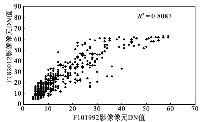
Fig. 2 The linear correlation of DN values between F101992 and F182012 night-time light images for the city of Hegang, in Heilongjiang Province图2 黑龙江省鹤岗市1992-2012年的F10与F18传感器夜间灯光影像像元DN值的线性相关关系 |
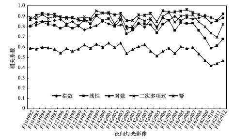
Fig. 3 The correlation coefficients (R2) for the five regression models图3 5种回归模型的相关系数 |
Tab. 1 Intercalibration model coefficients for each image表1 每一期影像的相互校正模型参数 |
| 卫星序号 | 年份 | a | b | R2 |
|---|---|---|---|---|
| F10 | 1992 | 0.6044 | 1.3244 | 0.8662 |
| 1993 | 0.7039 | 1.3265 | 0.9112 | |
| 1994 | 0.7654 | 1.2925 | 0.9265 | |
| F12 | 1994 | 0.6443 | 1.3133 | 0.9156 |
| 1995 | 0.8080 | 1.2227 | 0.9179 | |
| 1996 | 1.0288 | 1.1393 | 0.8972 | |
| 1997 | 0.7561 | 1.2646 | 0.8878 | |
| 1998 | 0.6846 | 1.2333 | 0.8880 | |
| 1999 | 0.7741 | 1.2315 | 0.8645 | |
| F14 | 1997 | 1.3708 | 1.1824 | 0.8579 |
| 1998 | 0.9664 | 1.2229 | 0.8663 | |
| 1999 | 1.0912 | 1.2263 | 0.9098 | |
| 2000 | 0.9913 | 1.1753 | 0.9308 | |
| 2001 | 0.8686 | 1.2266 | 0.9351 | |
| 2002 | 0.9894 | 1.1583 | 0.9153 | |
| 2003 | 0.9003 | 1.2019 | 0.9290 | |
| F15 | 2000 | 0.8093 | 1.1830 | 0.8592 |
| 2001 | 0.6655 | 1.2646 | 0.8619 | |
| 2002 | 0.5923 | 1.2795 | 0.9121 | |
| 2003 | 1.0439 | 1.1822 | 0.9111 | |
| 2004 | 1.1450 | 1.0847 | 0.9281 | |
| 2005 | 1.3548 | 1.0228 | 0.8498 | |
| 2006 | 1.2481 | 1.0738 | 0.9545 | |
| 2007 | 1.1421 | 1.1297 | 0.9384 | |
| F16 | 2004 | 0.7415 | 1.1576 | 0.9413 |
| 2005 | 0.9048 | 1.1776 | 0.9485 | |
| 2006 | 0.8296 | 1.1883 | 0.9647 | |
| 2007 | 0.7314 | 1.2132 | 0.9369 | |
| 2008 | 0.7927 | 1.1487 | 0.9186 | |
| 2009 | 0.6051 | 1.1525 | 0.8923 | |
| F18 | 2010 | 0.3427 | 1.2188 | 0.8387 |
| 2011 | 0.7035 | 1.0872 | 0.8545 | |
| 2012 | 0.4821 | 1.1866 | 0.8849 |
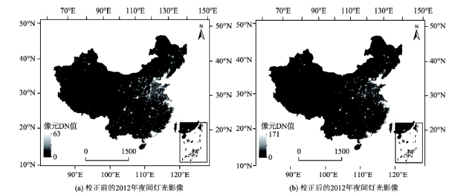
Fig. 4 The night-time light images of China图4 中国区域夜间灯光影像 |
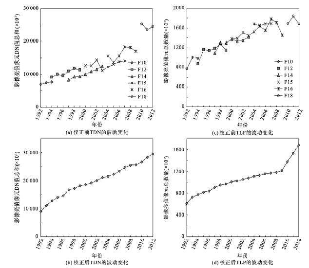
Fig. 5 The TDN and the TLP of the night-time light images before and after correction图5 校正前后夜间灯光数据的TDN和TLP |
Tab. 2 R2 of linear regression between the TDN and the corresponding GDP data at the provincial level表2 省级尺度上夜间灯光影像TDN与对应的GDP的线性回归的相关系数 |
| 年份 | 校正前 | 校正后 | |||||
|---|---|---|---|---|---|---|---|
| F10 | F12 | F14 | F15 | F16 | F18 | ||
| 1992 | 0.7096 | 0.7303 | |||||
| 1993 | 0.5953 | 0.6944 | |||||
| 1994 | 0.5979 | 0.6664 | 0.6546 | ||||
| 1995 | 0.6781 | 0.6850 | |||||
| 1996 | 0.6903 | 0.7272 | |||||
| 1997 | 0.7129 | 0.7201 | 0.7363 | ||||
| 1998 | 0.7208 | 0.7265 | 0.7388 | ||||
| 1999 | 0.7545 | 0.7641 | 0.7504 | ||||
| 2000 | 0.7100 | 0.7469 | 0.7595 | ||||
| 2001 | 0.7372 | 0.7373 | 0.7648 | ||||
| 2002 | 0.8086 | 0.7806 | 0.7898 | ||||
| 2003 | 0.8383 | 0.8482 | 0.8204 | ||||
| 2004 | 0.8338 | 0.7822 | 0.8238 | ||||
| 2005 | 0.7877 | 0.7636 | 0.8399 | ||||
| 2006 | 0.8110 | 0.7869 | 0.8446 | ||||
| 2007 | 0.8170 | 0.7908 | 0.8453 | ||||
| 2008 | 0.7784 | 0.8480 | |||||
| 2009 | 0.6904 | 0.8309 | |||||
| 2010 | 0.6964 | 0.8234 | |||||
| 2011 | 0.7755 | 0.8160 | |||||
| 2012 | 0.7293 | 0.7911 | |||||
Tab. 3 R2 of linear regression between the TDN per area and the corresponding GDP data per area at the prefecture level表3 市级尺度上夜间灯光影像单位面积的TDN与对应的单位的面积GDP的线性回归的相关系数 |
| 年份 | 校正前 | 校正后 | |||||
|---|---|---|---|---|---|---|---|
| F10 | F12 | F14 | F15 | F16 | F18 | ||
| 1992 | 0.6588 | 0.7094 | |||||
| 1993 | 0.6521 | 0.7069 | |||||
| 1994 | 0.6577 | 0.6572 | 0.7046 | ||||
| 1995 | 0.6337 | 0.6813 | |||||
| 1996 | 0.6266 | 0.6685 | |||||
| 1997 | 0.6114 | 0.6543 | 0.6526 | ||||
| 1998 | 0.6180 | 0.6632 | 0.6066 | ||||
| 1999 | 0.5717 | 0.6081 | 0.5955 | ||||
| 2000 | 0.6137 | 0.5877 | 0.6061 | ||||
| 2001 | 0.5429 | 0.5396 | 0.5613 | ||||
| 2002 | 0.4540 | 0.4235 | 0.4863 | ||||
| 2003 | 0.4452 | 0.4683 | 0.4799 | ||||
| 2004 | 0.4354 | 0.4076 | 0.4757 | ||||
| 2005 | 0.3766 | 0.3729 | 0.4299 | ||||
| 2006 | 0.3590 | 0.3393 | 0.4103 | ||||
| 2007 | 0.3406 | 0.3130 | 0.3914 | ||||
| 2008 | 0.3081 | 0.3866 | |||||
| 2009 | 0.3147 | 0.3875 | |||||
| 2010 | 0.2657 | 0.3877 | |||||
| 2011 | 0.2742 | 0.3846 | |||||
| 2012 | 0.2732 | 0.3955 | |||||
Tab. 4 R2 of linear regression between the TDN and the corresponding electric power consumption data at the province level表4 省级尺度上夜间灯光影像TDN与对应电力消耗值的线性回归的相关系数 |
| 年份 | 校正前 | 校正后 | |||||
|---|---|---|---|---|---|---|---|
| F10 | F12 | F14 | F15 | F16 | F18 | ||
| 1992 | - | - | |||||
| 1993 | - | - | |||||
| 1994 | - | - | - | ||||
| 1995 | 0.7578 | 0.7476 | |||||
| 1996 | - | - | |||||
| 1997 | - | - | - | ||||
| 1998 | - | - | - | ||||
| 1999 | 0.7858 | 0.8171 | 0.8207 | ||||
| 2000 | 0.7823 | 0.8135 | 0.8549 | ||||
| 2001 | 0.8231 | 0.8217 | 0.8648 | ||||
| 2002 | 0.8447 | 0.8323 | 0.8754 | ||||
| 2003 | 0.8608 | 0.8767 | 0.8791 | ||||
| 2004 | 0.8681 | 0.8030 | 0.8834 | ||||
| 2005 | 0.8272 | 0.8009 | 0.8819 | ||||
| 2006 | 0.8512 | 0.8402 | 0.8911 | ||||
| 2007 | 0.8577 | 0.8505 | 0.8985 | ||||
| 2008 | 0.8427 | 0.8980 | |||||
| 2009 | 0.7458 | 0.8902 | |||||
| 2010 | 0.7561 | 0.8789 | |||||
| 2011 | 0.8424 | 0.8759 | |||||
| 2012 | 0.8279 | 0.8704 | |||||
The authors have declared that no competing interests exist.
| [1] |
|
| [2] |
|
| [3] |
|
| [4] |
|
| [5] |
|
| [6] |
|
| [7] |
|
| [8] |
|
| [9] |
|
| [10] |
|
| [11] |
|
| [12] |
|
| [13] |
|
| [14] |
|
| [15] |
|
| [16] |
|
| [17] |
|
| [18] |
|
| [19] |
|
| [20] |
|
| [21] |
|
| [22] |
|
| [23] |
|
| [24] |
|
| [25] |
|
| [26] |
|
| [27] |
|
| [28] |
|
| [29] |
|
| [30] |
|
/
| 〈 |
|
〉 |
