遥感科学与应用技术

面向中尺度涡提取的SLA去噪方法研究

  • 吴书超 1, 2 ,
  • 董庆 , 1, * ,
  • 薛存金 1 ,
  • 毕经武 1, 2 ,
  • 廖志宏 1, 2 ,
  • 宋晚郊 1, 2
展开
  • 1. 中国科学院遥感与数字地球研究所 数字地球重点实验室,北京 100094
  • 2. 中国科学院大学,北京 100049
*通讯作者:董 庆(1965-),男,博士生导师,研究员,主要从事海洋遥感与全球变化领域研究。E-mail:

作者简介:吴书超(1990-),男,硕士生,主要从事海洋中尺度涡研究。E-mail:

收稿日期: 2016-04-07

  要求修回日期: 2016-04-24

  网络出版日期: 2016-09-27

基金资助

国家自然科学基金项目(41371385、41476154)

Denoising Algorithm of Sea Level Anomalies for Mesoscale Eddy Extraction

  • WU Shuchao 1, 2 ,
  • DONG Qing , 1, * ,
  • XUE Cunjin 1 ,
  • BI Jingwu 1, 2 ,
  • LIAO Zhihong 1, 2 ,
  • SONG Wanjiao 1, 2
Expand
  • 1. Key Laboratory of Digital Earth Sciences, Institute of Remote Sensing and Digital Earth, Chinese Academy of Sciences, Beijing 100094, China
  • 2. University of Chinese Academy of Sciences, Beijing 100049, China
*Corresponding author: DONG Qing, E-mail:

Received date: 2016-04-07

  Request revised date: 2016-04-24

  Online published: 2016-09-27

Copyright

《地球信息科学学报》编辑部 所有

摘要

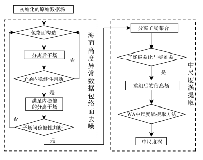
噪声去除一直是基于卫星高度计资料的海洋中尺度涡提取研究的难点和热点,然而无论是卷积滤波器还是信息滤波器都存在对海面高度异常(SLA)数据的局部过处理现象。鉴于此,本文提出一种基于包络面去噪的海洋中尺度涡提取方法。该算法可利用分离层内的信息稳定性和层间的信息完备性,很好地改进了卷积运算没有考虑局部噪声的不足,进而有效地提高去噪能力。其具体流程为:首先,对初始化的原始数据场进行上下包络面构造,形成原始数据子场;然后,根据子场内部和子场间的稳健性,把原始数据场转换为子场集合;其次,利用子场极差和标准差,对子场集合进行信息重组,形成噪声去除后的信息场;最后,利用去噪后的信息场数据,采用Winding-Angle(WA)和泛克立金中尺度涡提取算法在西北太平洋进行对比验证实验。实验结果表明,本文提出的方法较前人的方法有较大的提升,准确率为91.23%,取得了较好的应用效果。

本文引用格式

吴书超 , 董庆 , 薛存金 , 毕经武 , 廖志宏 , 宋晚郊 . 面向中尺度涡提取的SLA去噪方法研究[J]. 地球信息科学学报, 2016 , 18(9) : 1240 -1248 . DOI: 10.3724/SP.J.1047.2016.01240

Abstract

The noise removal of sea level anomaly (SLA) data set is crucial and important for extracting the mesoscale eddies. There are many filtering methods that have been developed for eliminating the noises in the sea level anomaly data set before extracting the mesoscale eddies. Nowadays, there are two mainstream approaches of noise removal, which are the convolution filtering and the information filtering. However, these filtering methods have some disadvantages that they could not recognize the right signal from the wrong signals. Therefore, some of the wrong or negligible signals are also taken into account by these noises removal methods. For solving this problem, an envelope surface-based denoising algorithm of sea level anomaly data is proposed before extracting the mesoscale eddies. The envelope surface-based denoising algorithm could improve the effect of noise removal by using the information stability and completeness in the separated layers. This algorithm overcomes the insufficiency of the convolution filtering method that it could not distinguish the wrong signal from the right ones. The detailed process of the envelope surface-based denoising algorithm includes three steps. First of all, the upper and lower envelope structures are used on the original data sets which have been initialized for extracting the subfields of sea level anomaly. Secondly, according to the robustness inside and among several subfields, the envelope surface-based denoising algorithm decomposes the original sea level anomaly fields into several subfields. The subfields could represent the information of the original sea level anomaly from different layers. Then the ranges and standard deviations of these subfields are adopted to recombine the information of several subfields set for shaping an information field after the noise removal. In the end, based on the information field after noise removal, the mesoscale eddies in the northwestern Pacific (22°N-50°N, 130°E-150°W) are extracted by applying the Winding-Angle (WA) algorithm. The results are compared with the mesoscale eddies extracted by the universal Kriging algorithm. From the results of this case study in the northwestern Pacific, we proved the veracity and efficiency of the envelope surface-based denoising algorithm. The veracity of the extracted mesoscale eddies could reach 91.23% in total. In contrary to the universal Kriging algorithm, the veracity of the extracted mesoscale eddies is greatly enhanced.

1 引言

中尺度涡是大洋中普遍存在的一种海洋涡流现象,它反映了海洋中各种物理变化的动力过程。海洋中尺度涡所蕴含的动能占全球海洋能量的80%以上,对海洋中物质能量的传输以及全球的气候变化具有重要影响[1-3]。因此,实现对中尺度涡的有效提取是开展各项海洋学研究和全球气候变化研究的关键。综合对地观测技术的发展,基于卫星高度计获取的海平面高度异常(Sea Level Anomaly,SLA)数据是目前海洋中尺度涡提取的常用解决方案。然而,一方面,SLA受卫星轨道参数偏差、传感器系统误差和大气等因素的影响[4-5],形成了SLA数据中的噪声信息,且SLA数据在生成过程中使用的多年统计参数也对SLA产品造成影响,进而影响了从SLA数据中提取中尺度涡的精度[6-8];另一方面,由地球自转和纬度差异变化引起的罗斯贝波的变形半径尺度与中尺度涡的空间尺度相近,这对中尺度涡的识别和提取造成干扰[9]。因此,去除其他引起海面高度异常的干扰和SLA数据中的噪声,是海洋中尺度涡提取的必要前提。
目前,根据不同滤波的原理,针对海洋中尺度涡提取的SLA数据滤波方法主要可分为卷积滤波和信息滤波2大类。卷积滤波方法主要从图形分析的角度出发,根据中尺度涡在SLA图像中表现的形态特征,建立针对中尺度涡的图形卷积算子,用于提取SLA数据中有效高频信息和滤除低频噪声信息。但由于中尺度涡在SLA图像中形态的多样性,单一的卷积算子在实际应用中很难做到全局的普适性。在一些局部区域的SLA去噪过程中,部分噪声没有得到有效剔除,反而通过卷积处理使噪声增强,进一步干扰了中尺度涡的识别和提取[10-12]。信息滤波方法是一种基于不同信息源特性实现有效信息和噪声分离的方法,其中采用傅里叶滤波对SLA数据进行频率域滤波,是该方法常用的滤波方式。该方法针对中尺度涡在频率域的特点,通过 设计高通滤波器来滤除低频噪声信息,进而增强SLA数据的中尺度涡信息。但是,该方法只能对 全局SLA数据进行去噪处理,对于局部空间的中 尺度涡特征的处理缺乏针对性,这导致部分区域 的提取结果与中尺度涡的实际分布存在较大的 偏差[13]
从上述分析可知,由于中尺度涡在SLA数据中具有复杂的空间和频率特性,导致利用中尺度涡的空间形态特征建立的卷积算子和利用中尺度涡的频率特征设计的信息滤波算子,往往容易忽略局部信号特征,造成中尺度涡信息的过度滤波,进而影响提取精度。在去噪过程中,为了更有效地保留SLA数据中的中尺度涡信息、增强中尺度涡的局部信号特征,本文提出了一种基于包络面[14-18]的SLA数据滤波方法。该方法针对中尺度涡在SLA数据场中的分布特征,建立一个与SLA场中曲面极值相切,并保留原始曲面变化趋势的包络面,利用对该包络面的优化来增强SLA数据中的中尺度涡信息,使局部的中尺度涡的信息能够得到更好地保留,以达到降低中尺度涡的局部误判率和提高提取精度的效果。

2 基于包络面的中尺度涡提取方法

2.1 方法流程

SLA数据去噪是提取中尺度涡前期的重要步骤。包络面去噪借鉴了几何学和信息学的优势,将原始数据从高频到低频信息进行有效地提取和分离。由于中尺度涡具有自身固有的频率域且相对集中,在去噪算法时,既要考虑特定的信号频率,又要考虑去噪方法的局部分辨能力。本文提出的包络面去噪方法无需任何先验知识,利用场内信息进行信号的提取、分离和重组,实现对原始数据的有效去噪。该方法的具体步骤为:(1)原始数据场初始化;(2)基于克里金[19-20]的上下包络面构造;(3)子场稳健性判断;(4)基于子场极差比和标准差的子场信息重组。图1为该算法的流程图,主要分为SLA数据的包络面去噪处理;基于已有算法的海洋中尺度涡提取2部分。
Fig. 1 Flowchart of the envelope surface-based noise removal method for extracting mesoscale eddies

图1 包络面去噪的海洋中尺度涡提取流程

2.2 基于包络面的SLA去噪

2.2.1 SLA数据原始场初始化
数据初始化的目的是获得适合的后期运算数据。数据初始化时输入栅格形式的SLA数据,设为height(x, y),该数据需要考虑在经纬向的分辨率差异。例如,对于0.25°×0.25°的逐天数据,其经纬向分辨率都是0.25°,但由于随着纬度的增加纬线圈周长变小,从地理坐标系转化为投影坐标系时需要考虑纬向分辨率的变化(经向分辨率恒定)。另外,为了便于后续的分离处理,本文设置了全局场gridPrimitive(x, y)和局部场grid(x, y)。在信息提取过程中,令gridPrimitive(x, y)=height(x, y);在局部场初始化时,令grid(x, y)= gridPrimitive(x, y)。
2.2.2 上下克立金包络面的构造
克立金插值算法是解决平面上取样不均匀的稀疏样点问题,SLA数据的极值点空间分布具有类似的稀疏特征。克立金插值算法通过不同方向、距离上空间变异性的准确度量实现邻近数据样点对于待估点的插值,故其是一种无偏最优估计的方法。对SLA数据的极值点进行插值后,将上下包络面构造方法应用于海面高度异常数据的极值,进而对冷暖涡进行有效的分离,分别构造出相应的暖涡场(上包络面)和冷涡场(下包络面)。
对SLA数据场取区域极值(式(1)、(2)),随后通过克立金插值得到上下克立金包络面(式(3)、(4)),及其平均值(式(5))。
LocalMax ( x , y ) = LocalMax ( grid ( x , y ) ) (1)
LocalMin ( x , y ) = LocalMin ( grid ( x , y ) ) (2)
LocalMaxGrid ( x , y ) = Interpolat ion ( LocalMax ( x , y ) ) (3)
LocalMinGrid ( x , y ) = Interpolat ion ( LocalMin ( x , y ) ) (4)
LocalMidGrid ( x , y ) = 1 2 [ LocalMaxGrid ( x , y ) + LocalMinGrid ( x , y ) ] (5)
式中:LocalMax(x,y)和LocalMin(x,y)表示为取区域极大值函数和区域极小值函数;Interpolation(x,y)表示为插值函数;LocalMaxGrid(x,y)与LocalMinGrid(x,y)为构造出的上下克立金包络面。
2.2.3 分离子场构造与内稳健性判定
通过从局部场中减去局部中间场LocalMidGrid(x,y)构造分离子场hi(x,y),如式(6)所示。
h i ( x , y ) = grid ( x , y ) - Lo cal MidGr id ( x , y ) (6)
对于已分离出i个子场的局部场,分离第i+1个子场时,局部场计算公式如式(7)所示。
grid ( x , y ) = girdPrimitive ( x , y ) - i = 1 k h i ( x , y ) (7)
由于分离子场并非全部满足内稳健性条件,因而实际计算时需要对分离子场的内稳健性进行判定。内稳健性的判断条件有3项:
(1)极值个数和正负等值线数是否相等或相近(式(8))。
1 - 0.05 Number ( Maxima ) + Number ( Minima ) Number ( Contour ( 0 + ) ) + Number ( Contour ( 0 - ) ) 1 + 0.05 (8)
式中:Number( )为取个数函数,如Number ( Maxima ) 为取极大值的个数;Contour(0+)和Contour(0-)分别为等值线值大于0和小于0的集合;0.05为本文可接受的误差范围,该方法认为其数值有5%的误差为可接受范围。
(2)LocalMidGrid(x,y)≈[0],表示局部中间场趋近于0。
(3)极大值个数和极小值个数之差绝对值小于等于二者最大值的10%(式(9)),此条件是宽松条件。
Number ( Maxima ) - Number ( Minima ) Max ( Number ( Maxima ) , Number ( Minima ) ) × 100 % 10 % (9)
式中:Number( )如式(8)所示,Max( )函数为取输入中最大值的函数;宽松条件是对条件(1)的放大,为了更好的容差,设置10%为宽松条件的范围。
hi(x,y)不满足上述所有的判据,则令grid(x,y)=hi(x,y),重新构造上下包络面构造,直到hi(x,y)满足以上判别条件为止。经过判别后得到的分离子场被认为满足内部稳健性。
2.2.4 分离子场间稳健性判定
为了确保分离子场间具有显著的差异性,通过子场间的稳健性以及剩余信息量的多少确定子场分离的停止条件。
(1)分离子场间稳健性判据如式(10)所示。
SDIndex = x y [ h k - 1 ( x , y ) - h k ( x , y ) ] 2 h k - 1 2 (10)
设定阈值ε,当SDIndex小于ε时,停止分解。实验表明,当ε取0.2-0.3时[17],分离子场稳健性好。
(2)剩余信息量判据如式(11)所示。
LocalMidGr id ( x , y ) = [ 0 ] (11)
当子场间的稳健性和剩余信息量符合以上条件时,场间达到稳健状态,此时停止分层处理;否则,需重新构造上下包络面。
2.2.5 信息重组
信息重组是将满足条件的分离子场进行重新组合的过程,其重组的依据为层极差比和层标准 差[21]。层极差比是指层内最大值与最小值之差的绝对值与原始数据最大值与最小值之差的绝对值的比值(式(12)),表示层间信息的相对量;层标准差是指层内数据的标准差(式(13)),表示层内的信息量。极差采用的是场内最大与最小值之差,由已知信息height(x,y)范围约(-8000,8000)(10-4 m),而中尺度涡振幅大多需要达到8 cm[22],且其他干扰波振幅大多集中在10 cm以下[23],此值设定根据实际情况进行适当调整适配,本文结合信息情况设定20%。当分层的极差与原始数据极差比大于20%且层内信息丰富时,认为中尺度涡信息是有效的,进而根据波和运动的叠加原理,将其组合成新的二维标量场。
Max ( h i ( x , y ) ) - Min ( h i ( x , y ) ) Max ( height ( x , y ) ) - Min ( height ( x , y ) ) × 100 % 20 % (12)
StandardDeviation = 1 N x y [ grid ( x , y ) - grid ( x , y ) ¯ ] 2 (13)
式中:hi(x,y)为第i分层;height(x,y)为原始场;Max( )、Min( )为取最大最小函数;grid(x,y)为每次运算的初始场; grid ( x , y ) ¯ 为初始场的平均值;N为场内网格的总个数。
为有效说明原始数据场到稳健性子场信息组合的计算流程,本文对2008年8月1日22°N~50°N,130°E~150°W范围内的SLA数据进行了子场分离和稳健性判断,得出前5个分离子场的场内稳定和场间稳定达到最优,结果如图2所示。
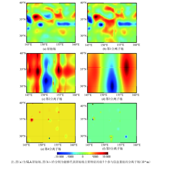
Fig. 2 The original field and decomposed subfields derived from envelope surface-based noise removal method

图2 SLA原始场和用包络面法得到的SLA分离子场。

5个分离子场的层标准差和极差比如表1所示。由表1可知,前3个分离子场所占原始数据量最大,且这3个子场的叠加场与原始数据的相关系数达到0.9437,能够代表原始数据的主要特征同时可减少参与计算的数据量。例如,图2(a)为海面高度异常的原始场;图2(b)-(f)分别为能够代表数据主要特征的前5个参与信息重组的分离子场,其中前3个子场中的数据差异较为显著,因而含有的信息量及空间频率也较大;图2(e)、(f)中包含的主要数据差异并不明显,且空间频率明显降低。因此,选择符合条件的前3个分离子场重组生成的新变量场就可能够很好地代表海面高度异常的主要信息,并滤除低频噪声的影响。
Tab. 1 Statistical results of the original field and the decomposed subfields (10-4 m)

表1 分场统计数据(10-4 m)

分场 极差比 标准差
第1分离子场 0.9788 482.3512
第2分离子场 0.2940 110.3303
第3分离子场 0.2134 41.3792
第4分离子场 0.0253 11.2313
第5分离子场 0.0057 6.4476
原始数据 1 477.0165
对分离子场和原始数据经过高通滤波处理后的场进行关联分析,结果表明第1分离子场同高斯滤波之后的结果相关系数达到0.9767,具有较高的相关性,进一步印证了包络面去噪方法在提取高频信息时具有更高的准确性。

2.3 海洋中尺度涡提取方法

由于基于流线几何的Winding-Angle(WA)[24]具有较高的中尺度涡提取准确率,而泛克立金中尺度涡提取算法[25]具有较强的去噪功能,故本文采用WA方法和泛克立金中尺度涡提取算法进行SLA去噪和中尺度涡提取的对比试验。
2.3.1 Winding-Angle(WA)算法
WA提取算法通过在SLA数据场内建立滑动窗口,寻找窗口内部的最小(最大)值点来判断可能的气旋涡(反气旋涡)中心,并由此为涡核向外扩展寻找流线或等值线,最外层流线或等值线即为涡旋的外缘线[26-27]。冷涡和暖涡的判别标准为:对于北半球,若涡旋中心的SLA比周围低,为气旋式涡旋(冷涡旋);若中心SLA比周围高,为反气旋式涡旋(暖涡旋)。WA方法提取中尺度涡主要使用流线的方式对中尺度涡识别,为保证涡旋的外边界连续,采用了曲线进行连接使其平滑。
2.3.2 泛克立金中尺度涡提取方法
泛克立金中尺度涡提取算法是运用变差函数工具计算SLA变差场,将变差场定义为广义振幅场,再利用泛克立金插值消除数据虚警和噪声,借助广义振幅场与实际振幅的关系通过少数几条特征等值线实现涡旋及其属性的提取。这种方法在提取中尺度涡前也需进行噪声剔除处理,与其他遥感提取方法的对比表明,北太平洋中尺度涡的成功识别率接近90%,过度识别率小于20%。

3 结果与讨论

3.1 数据来源及研究区

本文使用的SLA数据为法国AVISO(Archiving, Validation and Interpretation of Satellite Oceanographic Data)提供的TOPEX/Poseidon(T/P)、Jason、ERS1/2和Envisat等多种卫星观测数据融合的延时高度计产品,空间分辨率为0.25°×0.25°,时间分辨率为1 d。
研究区位于西北太平洋(22°N~50°N,130°E~150°W),选取黑潮活动较为强烈的区域(28°N~40°N,145°E~160°W)。时间范围为2008-2010年8-9月,该时间段西北太平洋地区的海洋活动强度相对 较高。

3.2 北太平洋局部区域的检测结果

对2008年8月1日22°N~50°N、130°E~150°W地区的SLA数据采用包络面方法去噪后,再利用WA方法提取得到中尺度涡空间分布图(图3)。西北太平洋黑潮等剧烈海洋运动的存在使得这个地区有较多的中尺度涡产生和发展。在经向上涡旋的分布呈现向东逐步减少的趋势;沿纬向呈现向北减少趋势,这与Chelton等和秦丽娟等28]等提取的中尺度涡在该地区的分布结果相似。
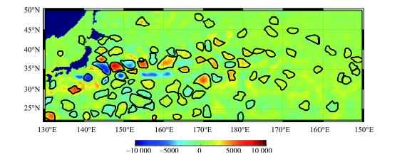
Fig. 3 Eddies extracted based on SLA dataset on August 1, 2008 (10-4 m)

图3 从2008年8月1日SLA数据集中提取得到的涡旋(10-4m)

图4为采用不同方法对2008年8月1日在局部区域(28°N~40°N,145°E~160°E)内提取中尺度涡的对比图。未采用包络面过滤的WA算法提取结果(图4(a))比通过滤波后的提取结果(图4(b))明显多提取了2个涡旋,剔除了一个涡旋。由此表明包络面去噪在涡旋活动剧烈区域对局部信息实现了增强,在涡旋活动和缓区对局部信息进行了有效滤波,去除了与中尺度涡不相干的信息,保留了关键信号,进而提高了中尺度涡的正确识别率。而通过卷积滤波的提取结果(图4(d)),出现了过度识别的现象和涡旋没有正确识别的现象,这与卷积滤波无差别增强信息特性有关,相比包络面过滤后提取结果较优。
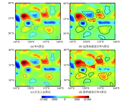
Fig. 4 Comparisons of eddies extracted by the WA method which is developed on the envelope surface-based noise-removal field (a), the original field (b), the universal Kriging algorithm (c), and the convolution noise removal field (d) respectively (10-4 m)

图4 中尺度涡提取对比结果(10-4m)

图4表明WA算法、包络面去噪的WA算法和泛克立金算法在中尺度涡提取结果上具有较高的一致性。另外,包络面去噪的WA算法可有效地去除信息中的噪声,而且该算法同泛克立金算法一样,具有对噪声信息滤除的作用。在本文实验中,泛克立金算法提取的涡旋边界明显比包络面去噪算法提取的中尺度涡边界小,出现了漏提取现象。这说明泛克立金算法在提取尺度大的涡旋时不会出现太大的偏差,而当处理相对小的涡旋时可能会出现漏提取的现象。图4中出现的涡旋耦合现象,是中尺度涡演变过程中时间序列上时刻的表现,原因可能是相互独立的2个涡旋近距离的相遇或者是2个涡旋合并(分裂)的中间某个时刻状态。基于包络面提取中尺度涡方法对耦合现象处理不仅依赖于周边海洋环境情况,还依赖边缘线的生成方法,该方法可很好地处理耦合现象,同时涡旋的耦合现象原因可以从中尺度涡长时间序列演变中得到确认和识别。

3.3 精度检验

考虑实验评价的客观性和准确性,本文对识别的结果进行了定量评价。依据Chaigneau等[13]所采用的识别结果定量评价方法,通过对比专家识别结果定量计算中尺度涡旋识别结果的准确程度。识别结果的定量评价方法有2个重要评价指标:正确识别率(Success of Detection Rate,SDR,式(14))和过度识别率(Excess of Detection Rate,EDR, 式(15))。
SDR = N c N e (14)
EDR = N om N e (15)
式中:SDR为正确识别率;Nc为包络面方法和其他方法共同提取出中尺度涡的数量;Ne为专家识别结果提取出中尺度涡的数量;EDR为过度识别率;Nom为本方法提取出但未被其他方法提取出的涡的数量。Chaigneau等[13]认为,过度识别率小于20%即为可接受误差的上限,满足此标准的方法,其识别精度即被认为达到实际研究要求。
在本文实验中,泛克立金中尺度涡提取算法较包络面法提取的涡旋边界小,说明前者使用的等值线围绕的区域面积相对较小,这可能导致提取的涡旋数量有所降低,然而包络面法识别出的区域面积相对较大,相对而言提取涡旋的过度识别率则会较高。由表2的精度检验结果可知,通过实验得出本方法的正确识别率为91.23%,过度识别率为14.01%,表明本文方法准确可行。
Tab. 2 Accuracy of eddies extracted by the proposed method

表2 包络面去噪提取中尺度涡的精度检验结果

数据时间 Ne Nc Nom SDR/(%) EDR/(%)
2008-08-01 10 10 2 100 20
2008-09-01 15 13 2 86.67 13.33
2009-08-01 17 16 3 94.12 17.67
2009-09-01 19 17 2 89.47 10.53
2010-08-01 18 16 3 88.89 16.67
2010-09-01 17 15 1 88.23 5.89
平均 - - - 91.23 14.01

4 结论

目前,广泛使用的AVISO SLA数据是在海面高度数据基础上去除平均海面高度、潮汐影响、大气压校正以及风与大气的高频响应校正后得到的数据,该数据包含多种噪声。在使用海面高度异常数据提取中尺度涡时,这些噪声会给中尺度涡提取精度带来不可忽视的影响,但对于如何过滤数据达到更好的提取精度,现有的解决方案仍存在不足。针对该问题,本文提出并实现了一种基于包络面的去噪滤波方法。该方法以统计学理论为基础,参与计算的参量少,具有较高的易操作性及普适性。通过在西北太平洋中尺度涡提取的对比实验,表明了该方法具有较高的实用性。主要结论如下:
(1)包络面法对海面高度异常数据具有明显的频率分离作用,可有效地分离提取出变量场的主要信息,分离后的信息从高频向低频过渡,数据信息量也逐层递减,能够准确地显示出海面高度异常数据的内在规律。
(2)包络面法得到的第1分离子场与高通滤波后的原始数据具有较高的相关性(相关系数为0.9767,且通过了95%的显著性检验),证实了包络面法去噪滤波后得到的第1分离子场有较高的空间频率。
(3)包络面法过滤后的数据能够更好地提取出局部小型涡旋,并且可以对大尺度非涡旋现象进行弱化滤波,能够根据空间频率局部调整数据趋势。该方法提取的中尺度涡准确率更高,滤波噪声效果更好,正确识别率达到91.23%。
(4)西北太平洋中尺度涡旋的提取试验表明,本文提出的方法准确率较传统方法提高了5.0%~15.0%,过度识别率降低了5%左右,表明本方法具有较好的应用效果。

The authors have declared that no competing interests exist.

[1]
Chelton D B, Schlax M G, Samelson R M.Global observations of nonlinear mesoscale eddies[J]. Progress in Oceanography, 2011,91(2):167-216.Sixteen years of sea-surface height (SSH) fields constructed by merging the measurements from two simultaneously operating altimeters are analyzed to investigate mesoscale variability in the global ocean. The prevalence of coherent mesoscale features (referred to here as "eddies") with radius scales of 0(100 km) is readily apparent in these high-resolution SSH fields. An automated procedure for identifying and tracking mesoscale features based on their SSH signatures yields 35,891 eddies with lifetimes >= 16 weeks. These long-lived eddies, comprising approximately 1.15 million individual eddy observations, have an average lifetime of 32 weeks and an average propagation distance of 550 km. Their mean amplitude and a speed-based radius scale as defined by the automated procedure are 8 cm and 90 km, respectively.<br/>The tracked eddies are found to originate nearly everywhere in the World Ocean, consistent with previous conclusions that virtually all of the World Ocean is baroclinically unstable. Overall, there is a slight preference for cyclonic eddies. However, there is a preference for the eddies with long lifetimes and large propagation distances to be anticyclonic. In the southern hemisphere, the distributions of the amplitudes and rotational speeds of eddies are more skewed toward large values for cyclonic eddies than for anticyclonic eddies. As a result, eddies with amplitudes >10 cm and rotational speeds >20 cm s(-1) are preferentially cyclonic in the southern hemisphere. By contrast, there is a slight preference for anticyclonic eddies for nearly all amplitudes and rotational speeds in the northern hemisphere.<br/>On average, there is no evidence of anisotropy of these eddies. Their average shape is well represented as Gaussian within the central 2/3 of the eddy, but the implied radius of maximum rotational speed is 64% smaller than the observed radius of maximum speed. In part because of this mismatch between the radii of maximum axial speed in the observations and the Gaussian approximation, a case is made that a quadratic function that is a very close approximation of the mode profile of the eddy (i.e., the most frequently occurring value at each radius) is a better representation of the composite shape of the eddies. This would imply that the relative vorticity is nearly constant within the interiors of most eddies, i.e., the fluid motion consists approximately of solid-body rotation.<br/>Perhaps the most significant conclusion of this study is that essentially all of the observed mesoscale features outside of the tropical band 20 degrees S-20 degrees N are nonlinear by the metric U/c, where U is the maximum circum-average geostrophic speed within the eddy interior and c is the translation speed of the eddy. A value of U/c > 1 implies that there is trapped fluid within the eddy interior. Many of the extratropical eddies are highly nonlinear, with 48% having U/c > Sand 21% having U/c > 10. Even in the tropics, approximately 90% of the observed mesoscale features are nonlinear by this measure.<br/>Two other nondimensional parameters also indicate strong degrees of nonlinearity in the tracked eddies. The distributions of all three measures of nonlinearity are more skewed toward large values for cyclonic eddies than for anticyclonic eddies in the southern hemisphere extratropics but the opposite is found in the northern hemisphere extratropics. There is thus a preference for highly nonlinear extratropical eddies to be cyclonic in the southern hemisphere but anticyclonic in the northern hemisphere.<br/>Further evidence in support of the interpretation of the observed features as nonlinear eddies is the fact that they propagate nearly due west with small opposing meridional deflections of cyclones and anticyclones (poleward and equatorward, respectively) and with propagation speeds that are nearly equal to the long baroclinic Rossby wave phase speed. These characteristics are consistent with theoretical expectations for large, nonlinear eddies. While there is no apparent dependence of propagation speed on eddy polarity, the eddy speeds relative to the local long Rossby wave phase speeds are found to be about 20% faster in the southern hemisphere than in the northern hemisphere. The distributions of the propagation directions of cyclones and anticyclones are essentially the same, except mirrored about a central azimuth angle of about 1.5 degrees equatorward. This small, but we believe statistically significant, equatorward rotation of the central azimuth may be evidence of the effects of ambient currents (meridional advection or the effects of vertical shear on the potential vorticity gradient vector) on the propagation directions of the eddies.<br/>While the results presented here are persuasive evidence that most of the observed westward-propagating SSH variability consists of isolated nonlinear mesoscale eddies, it is shown that the eddy propagation speeds are about 25% slower than the westward propagation speeds of features in the SSH field that have scales larger than those of the tracked eddies. This scale dependence of the propagation speed may be evidence for the existence of dispersion and the presence of features that obey linear Rossby wave dynamics and have larger scales and faster propagation speeds than the nonlinear eddies. The amplitudes of these larger-scale signals are evidently smaller than those of the mesoscale eddy field since they are not easily isolated from the energetic nonlinear eddies. (C) 2011 Elsevier Ltd. All rights reserved.

DOI

[2]
Yi J, Du Y, He Z, et al.Enhancing the accuracy of automatic eddy detection and the capability of recognizing the multi-core structures from maps of sea level anomaly[J]. Ocean Science, 2014,10(2):825-851.spatiotemporal model; identity-based change; composite object; interactions; ocean eddy

DOI

[3]
程旭华,齐义泉.基于卫星高度计观测的全球中尺度涡的分布和传播特征[J].海洋科学进展,2008,26(4):447-453利用将近12 a的融合高度计资料获得了全球海洋中尺度涡的空间分布和传播特

DOI

. [ Cheng X H, Qi Y Q.Distribution and propagation of mesoscale eddies in the global oceans learnt from altimetric data[J]. Advances in Marine Science, 2008,26(4):447-453. ]

[4]
Bronner E, Guillot A, Picot N.SARAL/AltiKa products handbook, Issue: 2 rev 4[R]. France, 2013.

[5]
Rio M H, Schaeffer P, Hernandez F, et al.The estimation of the ocean mean dynamic topography through the combination of altimetric data, in-situ measurements and GRACE geoid: from global to regional studies[C]. Proceedings of the GOCINA International Workshop, 2005.

[6]
Traon P Y L, Ogor F. ERS-1/2 orbit improvement using TOPEX/Poseidon: the 2 cm challenge[J]. Journal of Geophysical Research Atmospheres, 1998,103(3334):8045-8058.The ERS orbit error reduction method using TOPEX/POSEIDON (T/P) data as a reference [Le Traon et al., 1995a] was applied to ERS-1 cycles from phases C, E, F, and G and to the first 16 cycles of the ERS-2 mission (phase A). T/P M-GDR (geophysical data record) (version C) and ERS-1/2 ocean product (OPR) data were used. ERS-1/2 orbits are the D-PAF (processing and archiving facility) orbits and, when necessary, ERS-1/2 altimetric corrections were updated to make the T/P and ERS-1/2 corrections homogeneous. The adjustment method has been refined, and formal error on the estimation is now calculated. The ERS-1/2 orbit error estimation is thus estimated to be precise to within about 2 cm root-mean-square (rms). E-E crossover differences are reduced from 12 to 17 cm to only 6.5 cm rms for all processed cycles. Similarly, the T/P-E crossover differences are reduced from 11 to 14 cm to only 7 cm rms. The adjusted D-PAF orbit error varies between 6 and 12 cm rms. The adjustment has also been performed for the Joint Gravity Model 3(JGM 3) orbits of ERS-I phases C, E, and F. The rms difference between the corrected orbits for the D-PAF and JGM 3 orbits is only about 1 cm rms, while it is about 11 cm before T/P orbit error correction. This shows that the adjustment is almost insensitive to the initial ERS-I orbit used. It also confirms the 2 cm precision of the method. We also do repeat-track analysis on the 35 day repeat cycles of ERS-I phase C. The mean difference in sea level variance before and after orbit error correction is 34 cm2 (D-PAF orbit) and 17 cm2 (JGM 3 orbit). The corrected ERS-1 and T/P sea level variabilities, however, are in excellent agreement. The study thus shows that ERS-1/2 orbit error must be corrected before analyzing large-scale oceanic signals and combining ERS-1/2 with T/P data. The proposed method provides a very effective correction and thus significantly enhances the quality of ERS-1/2 data. Corresponding data sets will be distributed to the scientific community by Archiving, Validation, and Interpretation of Satellite Oceanographic Data (AVISO).

DOI

[7]
Traon P Y L, Faugère Y, Hernandez F, et al. Can we merge GEOSAT follow-on with TOPEX/Poseidon and ERS-2 for an improved description of the ocean circulation[J]. Journal of Atmospheric and Oceanic Technology, 2003,20(6):889-895.

[8]
Ducet N, Traon P Y L, Reverdin G. Global high resolution mapping of ocean circulation from TOPEX/Poseidon and ERS-1/2[J]. Journal of Geophysical Research Atmospheres, 2000,105(C8):19477-19498.

[9]
Stammer D.Global characteristics of ocean variability from regional TOPEX/POSEIDON altimeter measurements[J]. Journal of Physical Oceanography, 1997,27(8):1743-1769.Abstract Three years of altimetric data from the TOPEX/POSEIDON spacecraft have been used to study characteristics of eddy variability over the World Ocean. The nature of the variability and its spatial structure are characterized in terms of the geographical distribution of eddy energy, as simple approximations of observed regional frequency and wavenumber spectra, and in terms of associated eddy time and space scales of sea surface height (SSH) variability and geostrophic velocity. Emphasis is put on summarizing characteristics typical for dynamically distinct regions of the World Ocean. This effort results in an attempt to describe the observed ocean variability in terms of universal spectral relations that depend only on few mean flow parameters such as the first-mode Rossby radius of deformation. Regional peculiarities follow naturally as deviations from the fundamental frequency and wavenumber spectra presented here. Frequency spectra of both variables can be summarized by three basic types represen...

DOI

[10]
Chelton D B, Schlax M G, Lyman J M, et al.Equatorially trapped Rossby waves in the presence of meridionally sheared baroclinic flow in the Pacific Ocean[J]. Progress in Oceanography, 2003,56(2):323-380.TOPEX/POSEIDON altimeter data are analyzed for the 8.5-year period November 1992 to May 2001 to investigate the sea surface height (SSH) and geostrophic velocity signatures of quasi-annual equatorially trapped Rossby waves in the Pacific. The latitudinal structures of SSH and both components of geostrophic velocity are found to be asymmetric about the equator across the entire Pacific with larger amplitude north of the equator. The westward phase speeds are estimated by several different methods to be in the range 0.5-0.6 m s. These observed characteristics are inconsistent with the classical theory for first vertical, first meridional mode equatorially trapped Rossby waves, which predicts a phase speed of about 0.9 m swith latitudinally symmetric structures of SSH and zonal velocity and antisymmetric structure of meridional velocity. The observations are even less consistent with the latitudinal structures of SSH and geostrophic velocity components for other modes of the classical theory.The latitudinal asymmetries deduced here have also been consistently observed in past analyses of subsurface thermal data and altimeter data and have been variously attributed to sampling errors in the observational data, a superposition of multiple meridional Rossby wave modes, asymmetric forcing by the wind, and forcing by cross-equatorial southerly winds in the eastern Pacific. We propose a different mechanism to account for the observed asymmetric latitudinal structure of low-frequency equatorial Rossby waves. From the free-wave solutions of a simple 1.5-layer model, it is shown that meridional shears in the mean equatorial current system significantly alter the potential vorticity gradient in the central and eastern tropical Pacific. The observed asymmetric structures of sea surface height and geostrophic velocity components are found to be a natural consequence of the shear modification of the potential vorticity gradient. The mean currents also reduce the predicted westward phase speed of first meridional mode Rossby waves, improving consistency with the observations.

DOI

[11]
Pascual A, Faugère Y, Larnicol G, et al.Improved description of the ocean mesoscale variability by combining four satellite altimeters[J]. Geophysical Research Letters, 2006,33(2):356-360.1] Data from four satellite altimeters are combined with the aim of improving the representation of the mesoscale variability in the Global Ocean. All missions [Jason-1, ERS-2/ENVISAT, Topex/Poseidon interleaved with Jason-1 and Geosat Follow-On] are cross-calibrated previously to produce weekly gridded maps. In areas of intense variability, the rms differences between a classical configuration of two altimeters and the scenario merging four missions can reach 10 cm and 400 cm 2 /s 2 in SLA and EKE, respectively, which represents an important percentage of the signal variance. A comparison with surface drifters shows that the four altimeter scenario improves the recovery of mesoscale structures that were not properly sampled with Jason-1 + ERS-2/ENVISAT. Finally, the consistency between altimetric and tide gauge data is improved by about 25% when coastal sea level is estimated with 4 satellites compared to the results obtained with 2 altimeters.

DOI

[12]
Chelton D B, Schlax M G, Samelson R M, et al.Global observations of large oceanic eddies[J]. Geophysical Research Letters, 2007,34(15):L15606.Ten years of sea-surface height (SSH) fields constructed from the merged TOPEX/Poseidon (T/P) and ERS-1/2 altimeter datasets are analyzed to investigate mesoscale variability in the global ocean. The higher resolution of the merged dataset reveals that more than 50% of the variability over much of the World Ocean is accounted for by eddies with amplitudes of 5-25 cm and diameters of 100-200 km. These eddies propagate nearly due west at approximately the phase speed of nondispersive baroclinic Rossby waves with preferences for slight poleward and equatorward deflection of cyclonic and anticyclonic eddies, respectively. The vast majority of the eddies are found to be nonlinear.

DOI

[13]
Chaigneau A, Gizolme A, Grados C.Mesoscale eddies off Peru in altimeter records: identification algorithms and eddy spatio-temporal patterns[J]. Progress in Oceanography, 2008,79(2):106-119.We then investigate vortices off Peru using more than 20,000 mesoscale eddies identified by the winding-angle method. Coherent eddies, characterized by a high ratio of vorticity to deformation rate, are typically formed along the coast and propagate westward at 3–602cm02s 611 . The vortices have a mean radius of 8002km, increasing northward, and are most frequently observed off of Chimbote (9°S) and south of San Juan (15°S). The mean eddy lifetime is about 1 month, but if eddies survive at least 2 months, the probability for surviving an additional week (or month) is constant at 90% (or 67%). Anticyclonic eddies tend to propagate northwestward whereas cyclonic vortices migrate southwestward. In general, cyclones and anticyclones are similar, except for eddies surviving at least 6 months. In this case, after a similar 3–4 months of radius and amplitude growth, amplitudes (or sizes) decay particularly rapidly for anticyclonic (or cyclonic) eddies. In terms of intensity, cyclonic eddies show a rapid decay during the first 3 months before arriving at a quasi-constant value, whereas anticyclones exhibit steady decline. Finally, eddy temporal variations were examined at seasonal and interannual scales in the “coastal” region favorable to the formation of energetic mesoscale structures. On seasonal scales, eddy activity is maximal in fall and minimum in spring. At interannual scales, the eddy activity index was maximal during the strong El Ni09o of 1997–1998 but another strong maximum of eddy activity also occurred late in 2004. These temporal variations are probably associated with the intensification of the upwelling thermal front and with the passage of coastal-trapped waves which generate baroclinic instabilities. Further investigation of the mechanisms involved on the eddy genesis is needed.

DOI

[14]
朱乔. 数据包络分析(DEA)方法综述与展望[J].系统工程理论方法应用,1994(4):1-9.本文叙述了数据包络分析(DEA)方法的基本思想和模型,总结了近十多年来国内外的主要研究成果,并对该领域的进一步研究提出了一些想法和展望。

[ Zhu Q.Data envelopment analysis: a review and visions for future research[J]. System Engineering-Theory Methodology Applications, 1994,4:1-9. ]

[15]
陈一贤. HHT方法分析[D].杭州:浙江大学,2007. [ Chen Y X. Analysis of HHT[D]. Hangzhou: Zhejiang University, 2007. ]

[16]
孙加森. 数据包络分析(DEA)的交叉效率理论方法与应用研究[D].合肥:中国科学技术大学,2014.

[ Sun J S.Research on cross efficiency of data envelopment analysis (DEA): theoretical method and application[D]. Hefei: University of Science and Technology of China, 2014. ]

[17]
Rios R A, Parrott L, Lange H, et al.Estimating determinism rates to detect patterns in geospatial datasets[J]. Remote Sensing of Environment, 2015,156:11-20.The analysis of temporal geospatial data has provided important insights into global vegetation dynamics, particularly the interaction among different variables such as precipitation and vegetation indices. Nevertheless, this analysis is not a straightforward task due to the complex relationships among different systems driving the dynamics of the observed variables. Aiming at automatically extracting information from temporal geospatial data, we propose a new approach to detect stochastic and deterministic patterns embedded into time series and illustrate its effectiveness through an analysis of global geospatial precipitation and vegetation data captured over a 14 year period. By knowing such patterns, we can find similarities in the behavior of different systems even if these systems are characterized by different dynamics. In addition, we developed a novel determinism measure to evaluate the relative contribution of stochastic and deterministic patterns in a time series. Analyses showed that this measure permitted the detection of regions on the global map where the radiation absorbed by the vegetation and the incidence of rain occur with similar patterns of stochasticity. The methods developed in this study are generally applicable to any spatiotemporal data set and may be of particular interest for the analysis of the vast amount of remotely sensed geospatial data currently being collected routinely as part of national and international monitoring programs.

DOI

[18]
Mellado M, Tornero J.Object contour surface generation for robotic applications[C]. The 3rd IFAC/IFIP/IMACS Symposium, 1991.

[19]
Cressie N.Spatial prediction and ordinary kriging[J]. Mathematical Geology, 1988,20(4):405-421.

[20]
Pajak K, Glazer A.Semivariogram functions usage for a surface modeling with kriging method using data acquired with GNSS satellite method[C]. EGU General Assembly Conference Abstracts, 2013.

[21]
Hastie T, Tibshirani R, Friedman J, et al.The elements of statistical learning: data mining, inference and prediction[J]. The Mathematical Intelligencer, 2005,27(2):83-85.

[22]
林鹏飞. 南海和西北太平洋中尺度涡的统计特征分析[D].青岛:中国科学院研究生院(海洋研究所),2007.

[ Lin P F.Statistical analyses on mesoscale eddies in the South China Sea and the Northwest Pacific[D]. Qingdao: The Institute of Oceanology, Chinese Academy of Sciences, 2007. ]

[23]
Kantha L H, Clayson C A.Numerical models of oceans and oceanic processes[M]. Cambridge, MA: Academic Press, 2000.

[24]
Sadarjoen I A, Post F H.Geometric methods for vortex extraction[C]. Proceedings of the Joint Eurographics and IEEE TCVG Symposium on Visualization, 1999:53-62.

[25]
毕经武,董庆,薛存金,等.基于高度计遥感数据的北太平洋中尺度涡提取[J].遥感学报,2015,16(6):935-946.针对海洋中尺度涡现象,提出一 种基于海平面高度异常数据(SLA)的中尺度涡泛克里金提取算法。该算法运用变差函数工具计算SLA变差场,定义为广义振幅场,再利用泛克里金插值消除数 据虚警和噪声,借助广义振幅场与实际振幅的关系通过少数几条特征等值线实现涡旋及其属性的提取。选取北太平洋作为实验区,采用2012年4月的4期SLA 进行了中尺度涡的定量提取、分析,共提取出841个中尺度涡(含3个多核涡),包含450个气旋涡和391个反气旋涡;与其他遥感提取方法的对比显示北太 平洋中尺度涡的成功检测率接近90%,过度检测率小于20%。结果表明:(1)算法具有省时高效性,通过对SLA场的重构创建广义振幅场,避免了等值线筛 选过程,相对于海面高度闭合等值线等其他遥感方法具有判据简单及提取速度快的特性;(2)可靠性好,能够通过推导得出的特征等值线确保稳定的提取准确度; 算法建立在发展成熟的等值线提取方法之上,并且有变差函数与泛克里金法的理论支撑;(3)自适应性强,可以对任意海区进行实时的涡旋检测和提取,并且除振 幅值统计资料及必要基础数据外无需依赖其他辅助性数据。

DOI

[ Bi J W, Dong Q, Xue C J, et al.Extraction algorithm applied to northern Pacific mesoscale eddies based on altimetric remotely sensed data[J]. Journal of Remote Sensing, 2015,19(6):935-946. ]

[26]
Chaigneau A, Eldin G, Dewitte B.Eddy activity in the four major upwelling systems from satellite altimetry (1992-2007)[J]. Progress in Oceanography, 2009,83(1-4):117-123.Eddy activity in the four major eastern boundary upwelling systems (EBUS) is investigated using 15years of satellite altimetry data. Based on the analysis of more than 4000 long-lived eddy trajectories in every EBUS, we show that mesoscale structures are mainly generated along the continental coasts and south of the main archipelagos and propagate westward with velocities increasing toward the equator. These mesoscale eddies, having radii of 70鈥160km, are then frequently observed along the coastal transition zones and frontal regions and some large oceanic areas are preferentially populated by cyclonic or anticyclonic eddies. Temporal variations of the number of newly-formed eddies and the associated eddy activity index, defined as the mean eddy energy density, are finally examined at seasonal and interannual scales. The strongest seasonal (interannual, respectively) variations are observed in the California (Benguela) upwelling systems. The proposed indices also exhibit contrasted long-term trends in each EBUS, which suggests that eddy activity might be sensitive to a warming climate.

DOI

[27]
Chen G, Hou Y, Chu X.Mesoscale eddies in the South China Sea: mean properties, spatiotemporal variability, and impact on thermohaline structure[J]. Journal of Geophysical Research Oceans, 2011,116(C6):102-108.We investigated mean properties and the spatiotemporal variability of eddies in the South China Sea (SCS) by analyzing more than 7000 eddies corresponding to 827 eddy tracks, identified using the winding angle method and 17 years of satellite altimetry data. Eddies are mainly generated in a northeast-southwest direction and southwest of Luzon Strait. There is no significant difference between the numbers of two types of eddies (anticyclonic and cyclonic) in most regions. The mean radius and lifetime of eddies are 132 km and 8.8 weeks, respectively, both depending on where the eddies are formed. Anticyclonic and cyclonic eddies tend to deform during their lifetimes in different ways. Furthermore, eddy propagation and evolution characteristics are examined. In the northern SCS, eddies mainly propagate southwestward along the continental slope with velocities of 5.0-9.0 cm s(-1), while in the central SCS, eddies tend to move with slight divergence but still in a quasi-westward direction with velocities of 2.0-6.4 cm s(-1). Eddy propagation in the western basin to the east of Vietnam is quite random, with no uniform propagate direction. Investigation of 38 long-lived eddies shows that eddies have a swift growing phase during the first 12 weeks and then a slow decaying phase that affects the eddy radii and eddy energy densities. Nevertheless, vorticity has less variability. In addition, the effect of eddies on the thermocline and halocline is analyzed using 763 Argo temperature profile data. Cyclonic eddies drive the thermocline shallower and thinner and significantly strengthen the thermocline intensity, whereas anticyclonic eddies cause the thermocline to deepen and thicken and weaken the thermocline intensity to a certain degree. The halocline impacted by cyclonic eddies is also shallower and thinner than that impacted by anticyclonic eddies. Finally, eddy temporal variations are examined at seasonal and interannual scales. Eddy activity is sensitive to the wind stress curl and in the northern SCS it is also related with the strength of the background flows.

DOI

[28]
秦丽娟,董庆,樊星,等.卫星高度计的北太平洋中尺度涡时空分析[J].遥感学报,2015,19(5):806-817本文利用1993年—2012年AVISO卫星高度计融合数据,识别和追踪了北太平洋海域(100°E—77°W,0°N—70°N)20年的中尺度涡。统计分析了北太平洋中尺度涡的生命周期、振幅、移动速度等属性特征、空间分布和运动特征、季节、年际和年代际的变化趋势及其与ENSO的关系。结果表明:北太平洋中尺度涡的平均寿命为6.9周,平均振幅为8.44 cm,平均速度为6.4 cm/s;随着纬度的增加,反气旋涡的生命周期和振幅差异较大,气旋涡差异较小,涡旋的移动速度随纬度的增加逐渐减少。在空间分布上,日本东部的黑潮延伸区、加利福尼亚海岸和阿拉斯加湾是涡旋的高发区,其中黑潮延伸区分布最为密集;涡旋大多数向西运动,只有少数涡旋向东传播,移动过程中反气涡旋表现为向赤道方向偏移,气旋涡向极地方向偏移,且具有明显的非线性特征。在季节、年际尺度上,春季和夏季是涡旋高发的两个季节,秋季和冬季生成的涡旋相对最少,在加利福尼亚沿岸涡旋的季节差异较明显;涡旋数量的年际变化与ENSO事件具有明显的相关性,1993年—2002年厄尔尼诺年生成的涡旋较多,而拉尼娜年生成的涡旋较少,2003年—2012年则是厄尔尼诺年生成的涡旋较少,而拉尼娜年生成的涡旋较多。

DOI

. [ Qin L J, Dong Q, Fan X, et al.Temporal and spatial characteristics of mesoscale eddies in the North Pacific based on satellite altimeter data[J]. Journal of Remote Sensing, 2015,19(5):806-817. ]

文章导航

/