
顾及风向和风速的空气污染物浓度插值方法
作者简介:李佳霖(1992-),男,山东滨州人,硕士生,主要从事时空插值方法的研究工作。E-mail:garlic_lee@csu.edu.cn
收稿日期: 2016-05-09
要求修回日期: 2016-09-22
网络出版日期: 2017-03-20
基金资助
国家“863”计划(2013AA122301)
高等学校博士点专项科研基金(20110162110056)
湖南省博士生优秀学位论文资助项目(CX2014B050)
A Method of Spatial Interpolation of Air Pollution Concentration Considering WindDirection and Speed
Received date: 2016-05-09
Request revised date: 2016-09-22
Online published: 2017-03-20
Copyright
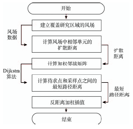
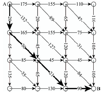
随着经济的快速发展,中国大部分地区空气污染状况日趋严重。空气污染物浓度插值对于进一步分析污染物时空分布情况,估计不同地区人群的暴露风险,制定防范措施具有重要作用。然而,现有空间插值方法由于没有充分考虑风向和风速因素对于污染物扩散的影响,故直接应用于空气污染物浓度插值,会对插值结果造成不利的影响。因此,本文提出一种顾及风向和风速的空气污染物浓度插值方法(Direction-Velocity IDW,DVIDW)。该方法首先根据离散气象站点处的风向和风速数据建立风场表面,然后利用风场数据计算空气污染物的扩散距离,根据扩散距离计算风场中待求点与采样点间的最短路径距离,最后由最短路径距离替代欧式距离进行反距离加权插值。本文分别采用2组实际空气污染物浓度数据,对DVIDW方法和其他常用的空间插值方法进行实验对比分析,验证了本文方法的可行性和优越性。
李佳霖 , 樊子德 , 邓敏 . 顾及风向和风速的空气污染物浓度插值方法[J]. 地球信息科学学报, 2017 , 19(3) : 382 -389 . DOI: 10.3724/SP.J.1047.2017.00382
With the rapid development of economy, air pollution becomes more and more serious in China. The quality of the interpolation results of air pollutant concentration is very significant for analyzing the spatial-temporal distribution of the air pollutant, estimating the exposure risk of people in different areas, and making precaution. However, there are some problems when applying the existing spatial interpolation methods directly to the interpolation of air pollutant concentration. One of the most important problems is that the existing spatial interpolation methods cannot fully consider the influence of wind direction and speed on the air pollutant diffusion. We proposed a method (Direction-Velocity IDW) of spatial interpolation of air pollutant concentration taking wind direction and speed into account. First, we constructed a wind-field surface based on the discrete wind direction and speed data and the diffusion distance is computed in the wind-field. Then, we used Dijkstra algorithm to obtain the shortest path in wind-field. Finally, we interpolated the attribute value using IDW by the shortest path distance instead of the Euclidean distance. In the experiment, we verified the effectiveness of the method we proposed by comparing DVIDW and the commonly used spatial interpolation methods. We concluded that the proposed method (DVIDW) can produce interpolation results with higher precision.
Fig. 1 Flow chart of the DVIDW algorithm图1 DVIDW算法流程图 |
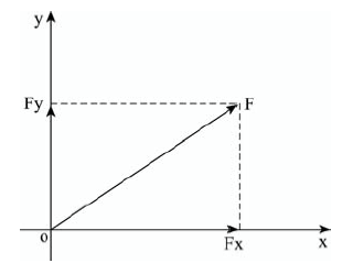
Fig. 2 Decomposition of vector data图2 矢量数据的分解 |
Fig. 3 The calculation of the shortest path in the wind field图3 风场最短路径计算 |
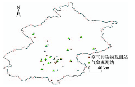
Fig. 4 The distribution map of air pollutant observation stations and meteorological observation stations图4 空气污染物观测站点和气象观测站点分布图 |
Tab. 1 Results of experiments by the four different spatial interpolation methods (Test 1)表1 4种空间插值方法实验结果(实验1) |
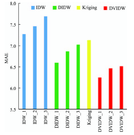
| MAE/(μg/m3) | RMS/(μg/m3) | |
|---|---|---|
| IDW_1 | 7.2732 | 15.2666 |
| IDW_2 | 7.4573 | 16.0977 |
| IDW_3 | 7.6951 | 17.0742 |
| DIDW_1 | 6.6000 | 14.5153 |
| DIDW_2 | 6.8691 | 14.8112 |
| DIDW_3 | 7.0291 | 15.0007 |
| Kriging | 7.1302 | 15.0958 |
| DVIDW_1 | 6.2557 | 14.5614 |
| DVIDW_2 | 6.4666 | 14.6923 |
| DVIDW_3 | 6.5208 | 14.7595 |
Fig. 5 Results of experiments by the four differentspatial interpolation methods (Test 1)图5 4种空间插值方法实验结果柱状图(实验1) |
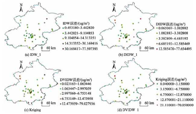
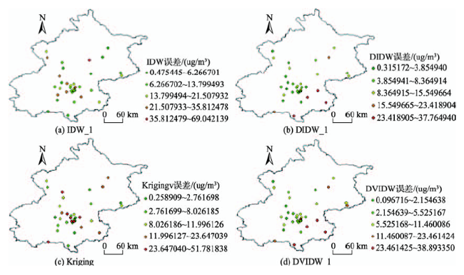
Fig. 6 The spatial distribution of results of four interpolation methods (Test 1)图6 4种方法插值结果误差空间分布(实验1) |
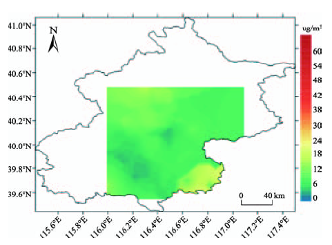
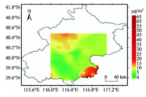
Fig. 7 The map of PM2.5 concentration interpolationresults图7 PM2.5浓度插值结果图 |
Tab. 2 Results of experiments by the four different spatial interpolation methods表2 4种空间插值方法的实验结果(实验2) |
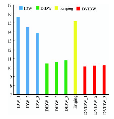
| MAE/(μg/m3) | RMS/(μg/m3) | |
|---|---|---|
| IDW_1 | 15.6575 | 20.2964 |
| IDW_2 | 14.5205 | 19.5501 |
| IDW_3 | 13.8425 | 19.1654 |
| DIDW_1 | 10.4757 | 14.5905 |
| DIDW_2 | 10.6549 | 14.6874 |
| DIDW_3 | 10.8367 | 14.8179 |
| Kriging | 15.1735 | 19.8676 |
| DVIDW_1 | 10.1501 | 14.6334 |
| DVIDW_2 | 10.2418 | 14.6044 |
| DVIDW_3 | 10.2829 | 14.5789 |
Fig. 8 Results of experiments by the six differentspatial interpolation methods (Test 2)图8 4种空间插值方法的实验结果柱状图(实验2) |
Fig. 9 The spatial distribution of results of four interpolation methods (Test 2)图9 4种方法插值结果误差的空间分布(实验2) |
Fig. 10 The map of PM2.5 concentration interpolation results图10 PM2.5浓度插值结果图 |
The authors have declared that no competing interests exist.
| [1] |
|
| [2] |
|
| [3] |
|
| [4] |
|
| [5] |
|
| [6] |
|
| [7] |
|
| [8] |
|
| [9] |
|
| [10] |
|
| [11] |
[
|
| [12] |
|
| [13] |
|
| [14] |
|
| [15] |
|
| [16] |
|
| [17] |
|
| [18] |
|
| [19] |
|
| [20] |
|
| [21] |
|
/
| 〈 |
|
〉 |