
基于多尺度对比学习的弱监督遥感场景分类
|
彭 瑞(1998— ),男,湖南常德人,硕士生,主要从事深度学习与遥感影像智能理解、地表异常即时探测等方面研究。E-mail: pengrui@mail.bnu.edu.cn |
收稿日期: 2021-12-15
修回日期: 2022-03-13
网络出版日期: 2022-09-25
基金资助
国家自然科学基金项目(42192584)
北京市自然科学基金项目(4214065)
Multi-Scale Contrastive Learning based Weakly Supervised Learning for Remote Sensing Scene Classification
Received date: 2021-12-15
Revised date: 2022-03-13
Online published: 2022-09-25
Supported by
National Natural Science Foundation of China(42192584)
Natural Science Foundation of Beijing Province(4214065)
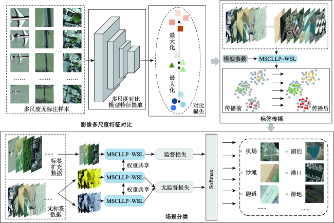
遥感场景分类作为一种理解遥感影像的重要方式,在目标检测、影像快速检索等方向有着重要的应用,当前主流的场景分类方法多关注影像深层次特征的准确提取,忽略了场景目标在不同分布尺度下的差异性。此外,有限的高质量场景标签进一步限制了模型分类性能。为了解决以上问题,本研究提出了基于多尺度对比学习的弱监督遥感场景分类方法,首先利用多尺度对比学习的自监督策略,从大量无标注数据中自动获取影像不同尺度下的特征表示。其次,基于多尺度稳健特征对分类模型利用少量标签进行微调,并结合标签传播方法生成高质量样本标签。最后,结合大量无标签数据构建弱监督分类模型,进一步提升场景分类的能力。本研究在遥感场景AID数据集和NWPU-RESISC45数据集上分别使用1%、5%和10%的标注样本下分类精度分别达到了87.7%、93.67%、95.56%和86.02%、93.15%和95.38%,在有限标注样本条件下与其他基准模型相比有着明显的优势,证明了本文模型的有效性。

彭瑞 , 赵文智 , 张立强 , 陈学泓 . 基于多尺度对比学习的弱监督遥感场景分类[J]. 地球信息科学学报, 2022 , 24(7) : 1375 -1390 . DOI: 10.12082/dqxxkx.2022.210809
Remote sensing scene classification is a significant approach to comprehending remote sensing images and has several applications in the areas such as target recognition and quick image retrieval. Currently, although many deep-learning-based scene classification algorithms have achieved excellent results, these methods only extract deep features of scene images on a specific scale and ignore the instability of extracted scene image features at different scales. Furthermore, the shortage of annotation data limits the performance improvement of these scene classification methods, which remains unsolved. As a result, for multi-scale remote sensing scene classification with limited labels, this article proposes a Multi-Scale Contrastive Learning Label Propagation based Weakly Supervised Learning (MSCLLP-WSL) approach. Firstly, a multi-scale contrastive learning method is utilized which effectively improves the ability of the model to obtain invariant features of scene images at different scales. Secondly, to address the problem of insufficient reliable labels, inspired by the Weakly Supervised Learning (WSL) method which supports a small number of labeled data and unlabeled data for training at the same time, this research further introduces WSL methods to make full use of the limited labels that exist in the data usage and production process. Label propagation is also used in this study to complete the tasks of annotating unlabeled data, which improves the performance of the proposed scene classification model even further. The proposed MSCLLP-WSL method has been extensively tested on the AID dataset and the NWPU-RESISC45 dataset with limited annotated data and compared with other benchmark algorithms named finetuned VGG16, finetuned Wideresnet50, and Skip-Connected Covariance (SCCov) network. Experiments demonstrate that multi-scale comparative learning enhances label propagation accuracy, which further improves the classification precision of complicated scenes with limited labeling samples. Hence, we set 1%, 5%, and 10% annotated data to represent the case of limited labels, accordingly. The results demonstrate that the proposed MSCLLP-WSL method in this study achieves an overall accuracy of 85.85%, 93.94%, and 95.65% on the AID dataset using 1%, 5%, and 10% labeled samples, respectively. Similarly, on the NWPU-RESISC45 dataset, the overall classification accuracy of 1%, 5%, and 10% annotated samples reaches 87.83%, 93.67%, and 95.47%, respectively. Although the overall accuracy of the latter dataset is lower than the former, the smaller amount of misclassification also indicates the stability of our proposal in the scene classification of large-scale datasets. The experiments results show that our proposed method achieves impressive performance on these two large-scale scenes datasets with limited annotated samples, which outperforms the benchmark methods in this article.
表1 数据集Tab. 1 Dataset |
| 数据集名称 | AID | NWPU-RESISC45 |
|---|---|---|
| 类别数 | 30 | 45 |
| 单类别影像数/个 | 220~420 | 700 |
| 空间分辨率/m | 8~0.5 | 30~0.2 |
| 影像尺寸 | 600×600 | 256×256 |
| 影像总数/张 | 10 000 | 31 500 |
|
| 算法1 MSCLLP-WSL模型 |
|---|
| 输入: 有标签场景数据集 , 无标签场景数据集 , 初始化自动编码器E和投影函数P,构建多尺度对比模型 多尺度对比学习: 1.构建同一尺度影像正负样本对 , 和 2.获取样本深度特征 、 和 3.使用式(2),计算 、 , 和相似程度 4.利用式(3)与式(4),计算所有正负样本相似度,构建对比损失函数 5.构建多尺度对比损失函数 6.多尺度对比模型 更新参数至 高置信标签传播下的弱监督遥感场景分类: 7.模型 构建标签传播模型 ,初始参数 8. , 训练模型 ,参数 更新至 9.如式(6)和式(7),当 , 10. 扩充标注样本集 至X 11. 构建弱监督场景分类模型 ,初始参数为 12.样本集X以及 训练模型 13.模型 训练完成 输出:无标注场景影像的标签 |
表2 尺度个数参数N对标签传播的精度影响Tab. 2 The effect of the number of scales parameter on the accuracy of label propagation |
| 尺度个数参数 | |||||
|---|---|---|---|---|---|
| N=1 | N=2 | N=3 | N=4 | N=5 | |
| 精度 | 0.7085 | 0.7093 | 0.71288 | 0.7031 | 0.6873 |
| 训练时长/h | 1.24 | 2.36 | 3.40 | 4.40 | 6.00 |
表3 不同比例无标注样本模型分类精度Tab. 3 Classification accuracy at different ratio of unlabeled sample |
| 无标注样本 | |||||||||
|---|---|---|---|---|---|---|---|---|---|
| 10% | 20% | 30% | 40% | 50% | 60% | 70% | 80% | 90% | |
| 分类精度/% | 82.94 | 83.88 | 84.2 | 85.16 | 85.7 | 85.72 | 84.85 | 85.83 | 84.74 |
表4 Vgg16、Wideresnet50和SCCov模型训练参数设置Tab. 4 Training Parameters setting of Vgg16, Wideresnet50 and SCCov model |
| 基准模型 | 迭代次数 | 批尺寸 | 标注样本 | 学习率 | 权重衰减 | 优化方法 | 参数量 |
|---|---|---|---|---|---|---|---|
| Vgg16 | 800(Epoch) | 20 | 1%/5%/10% | 0.001 | 0.0005 | SGD | 138M |
| Wideresnet50 | 800(Epoch) | 20 | 1%/5%/10% | 0.001 | 0.0005 | SGD | 67M |
| SCCov(Vgg16) | 200(Epoch) | 64 | 1%/5%/10% | 0.001 | 0.0005 | Adagrad | 13M |
表5 AID数据集上不同模型获取的总体精度结果比较Tab. 5 Comparison of OA(%) results obtained by different models on the AID dataset |
| 主干网络 | 方法 | 总体精度OA (Avg±Std)/ % | ||
|---|---|---|---|---|
| 1%标注样本 | 5%标注样本 | 10%标注样本 | ||
| VGG16 | 微调 | 49.05±2.39 | 79.06±0.85 | 86.86±1.03 |
| Wideresnet50 | 微调 | 63.05±1.84 | 84.72±0.8 | 89.75±0.4 |
| VGG16 | SCCov | 51.38±0.16 | 81.8±0.76 | 85.85±1.27 |
| Wideresnet50 | 本文模型 | 85.85±1.95 | 93.94±0.67 | 95.65±0.42 |
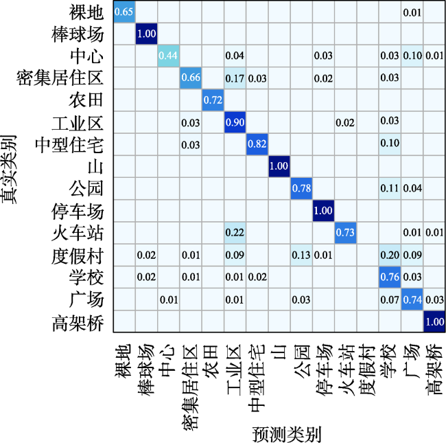
图4 AID数据集1%标注样本下部分类别混淆矩阵Fig. 4 Confusion matrix of partial categories under 1% labeled sample of AID dataset |
表6 AID数据集10%标注样本下单类别分类精度Tab. 6 Classification accuracy of each category under 10% labeled samples in the AID dataset |
| 类别 | 精度 | 类别 | 精度 | 类别 | 精度 | 类别 | 精度 | 类别 | 精度 |
|---|---|---|---|---|---|---|---|---|---|
| 机场 | 0.991 | 教堂 | 0.931 | 工业区 | 0.974 | 操场 | 1 | 学校 | 0.878 |
| 裸地 | 0.978 | 商业区 | 0.962 | 草地 | 0.976 | 池塘 | 0.968 | 稀疏住宅 | 0.989 |
| 棒球场 | 0.970 | 密集居住区 | 0.943 | 中型住宅 | 0.967 | 港口 | 1 | 广场 | 0.838 |
| 沙滩 | 0.983 | 沙漠 | 0.989 | 山 | 1 | 火车站 | 0.885 | 体育馆 | 0.977 |
| 桥梁 | 1 | 农田 | 0.982 | 公园 | 0.962 | 度假村 | 0.770 | 储罐 | 0.972 |
| 中心 | 0.808 | 森林 | 0.973 | 停车场 | 1 | 河流 | 0.976 | 高架桥 | 1 |
表7 NWPU-RESISC45数据集上不同模型获取的总体精度结果比较Tab. 7 Comparison of overall accuracy results obtained by different models on the NWPU-RESISC45 dataset |
| 主干网络 | 方法 | 总体精度OA (Avg±Std)/% | ||
|---|---|---|---|---|
| 1%标注样本 | 5%标注样本 | 10%标注样本 | ||
| VGG16 | 微调 | 51.73 ± 3.18 | 80.18 ± 0.63 | 85.89 ± 0.64 |
| Wideresnet50 | 微调 | 68.03 ± 0.73 | 84.06 ± 0.08 | 89.35 ± 0.36 |
| VGG16 | SCCov | 63.80 ± 1.04 | 85.62 ± 0.40 | 89.20 ± 0.60 |
| Wideresnet50 | 本文模型 | 87.38±0.61 | 93.67±0.20 | 95.47±0.17 |
注:蓝色加粗内容表示本文模型对比基准模型达到了最优。 |
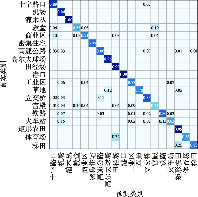
图6 NWPU-RESISC45数据集1%标注样本下部分类别混淆矩阵Fig. 6 Confusion matrix of partial categories under 1% labeled sample of NWPU-RESISC45 dataset |
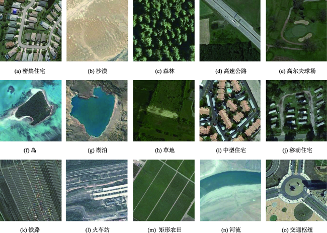
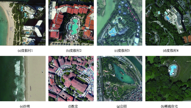
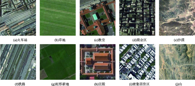
图7 NWPU-RESISC45数据集中相似场景示例Fig. 7 Examples of similar scenes in the NWPU-RESISC45 dataset |
表8 NWPU-RESISC45数据集10%标注样本下单类别分类精度Tab. 8 Classification accuracy of each category under 10% labeled samples in the NWPU-RESISC45 dataset |
| 类别 | 精度 | 类别 | 精度 | 类别 | 精度 | 类别 | 精度 | 类别 | 精度 |
|---|---|---|---|---|---|---|---|---|---|
| 十字路口 | 0.976 | 圆形农田 | 0.986 | 港口 | 0.981 | 宫殿 | 0.776 | 船 | 0.986 |
| 飞机 | 0.986 | 云 | 0.995 | 工业区 | 0.962 | 停车场 | 0.967 | 雪山 | 0.971 |
| 机场 | 0.962 | 商业区 | 0.933 | 岛 | 0.971 | 铁路 | 0.910 | 稀疏住宅 | 0.943 |
| 棒球场 | 0.990 | 密集住宅 | 0.890 | 湖泊 | 0.943 | 火车站 | 0.914 | 体育场 | 0.981 |
| 篮球场 | 0.981 | 沙漠 | 0.914 | 草地 | 0.910 | 矩形农田 | 0.924 | 储罐 | 0.990 |
| 海滩 | 0.948 | 森林 | 0.976 | 中型住宅 | 0.924 | 河流 | 0.967 | 网球场 | 0.976 |
| 桥梁 | 0.938 | 高速公路 | 0.848 | 移动住宅 | 1.000 | 交通枢纽 | 0.990 | 梯田 | 0.981 |
| 灌木丛 | 1.000 | 高尔夫球场 | 0.986 | 山 | 0.971 | 跑道 | 0.952 | 火电站 | 0.971 |
| 教堂 | 0.905 | 田径场 | 0.971 | 立交桥 | 0.976 | 海冰 | 0.971 | 湿地 | 0.843 |
| [1] |
|
| [2] |
|
| [3] |
|
| [4] |
|
| [5] |
|
| [6] |
|
| [7] |
|
| [8] |
|
| [9] |
|
| [10] |
|
| [11] |
|
| [12] |
何小飞, 邹峥嵘, 陶超, 等. 联合显著性和多层卷积神经网络的高分影像场景分类[J]. 测绘学报, 2016, 45(9):1073-1080.
[
|
| [13] |
郑海颖, 王峰, 姜维, 等. 神经网络训练策略对高分辨率遥感图像场景分类性能影响的评估[J]. 电子学报, 2021, 49(8):1599-1614.
[
|
| [14] |
钱晓亮, 李佳, 程塨, 等. 特征提取策略对高分辨率遥感图像场景分类性能影响的评估[J]. 遥感学报, 2018, 22(5):758-776.
[
|
| [15] |
|
| [16] |
|
| [17] |
|
| [18] |
|
| [19] |
|
| [20] |
|
| [21] |
|
| [22] |
|
| [23] |
|
| [24] |
|
| [25] |
|
| [26] |
|
| [27] |
|
| [28] |
|
| [29] |
|
| [30] |
|
| [31] |
|
| [32] |
|
| [33] |
|
| [34] |
|
| [35] |
|
| [36] |
|
| [37] |
|
| [38] |
|
| [39] |
|
/
| 〈 |
|
〉 |