
基于移动监测数据的不同城市场景下PM2.5浓度精细模拟与时空特征解析
|
谢晓苇(1997— ),男,福建永泰人,硕士生,主要从事地理信息资源环境分析研究。E-mail: n195520021@fzu.edu.cn |
收稿日期: 2021-12-23
修回日期: 2022-02-08
网络出版日期: 2022-10-25
基金资助
中国科学院战略性先导科技专项(A类)(XDA23100502)
Fine Simulation and Analysis of Temporal and Spatial Characteristics of PM2.5 Concentration Distribution in Different Urban Scenarios based on Mobile Monitoring Data
Received date: 2021-12-23
Revised date: 2022-02-08
Online published: 2022-10-25
Supported by
Strategic Priority Research Program of the Chinese Acadamic of Science(XDA23100502)
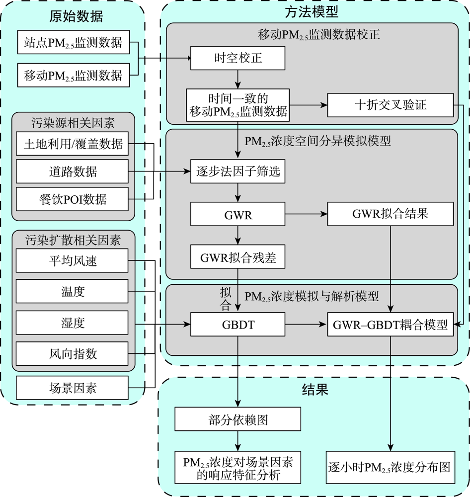
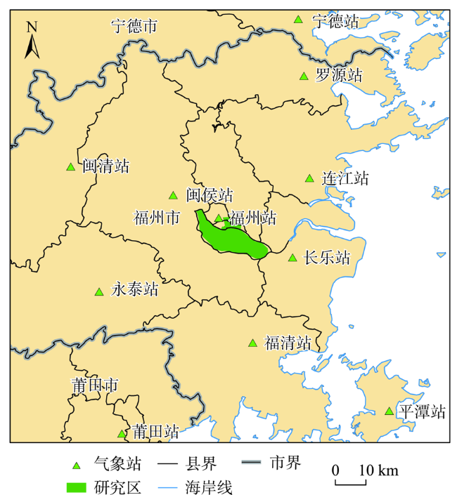
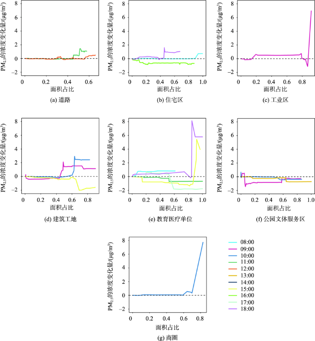
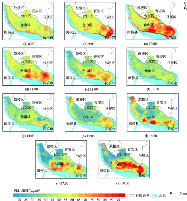
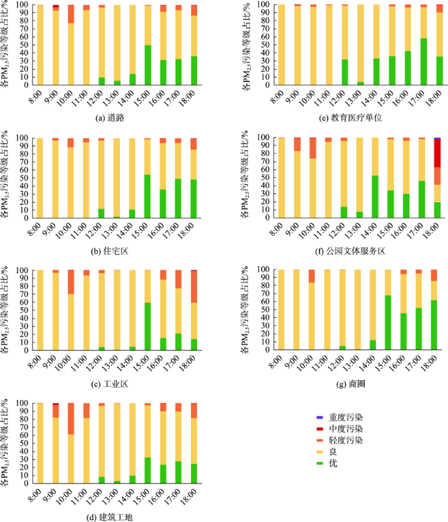
城市内部PM2.5浓度分布具有明显的空间异质性,而传统方法基于遥感数据或监测站点数据进行分析,难以揭示高时空分辨率下城市内部的PM2.5浓度分布特征,缺少不同时刻城市场景(如:道路、工业区、住宅区等)对PM2.5浓度复杂非线性影响的解析。本研究将移动监测传感器安装于快递车上,采集福州市主城区南部不同类型场景的PM2.5浓度,然后融合地理加权回归(Geographical Weighted Regression, GWR)和梯度提升决策树(Gradient Boosting Decision Tree, GBDT)方法,提出一种基于GWR-GBDT的PM2.5模拟与场景解析模型,能够较好地拟合气象、场景因素与PM2.5浓度的非线性关系,提升了城市PM2.5污染精细监测能力;并结合部分依赖图解析不同时段不同场景因素对PM2.5浓度的非线性作用影响。结果表明:① 基于移动PM2.5浓度监测数据,利用GWR-GBDT模型能够较好地模拟城市场景、气象和PM2.5浓度之间的非线性关系,能够有效精细模拟PM2.5浓度的空间分布,十折验证R2结果为0.52~0.94;② 通过部分依赖图分析同一场景在不同时段对PM2.5浓度响应的异质性,发现各类场景对PM2.5浓度提升或抑制作用并不稳定;③ 解析不同时段人类活动与城市场景对PM2.5浓度的交互作用发现,教育医疗单位和住宅区两类场景对PM2.5浓度的提升作用都与人类通勤有密切关系,高污染场景中的建筑工地在采取的洒水降尘措施后能在数小时内有效缓解PM2.5污染,公园文体服务区在多数时段对PM2.5浓度具有抑制作用,工业区和道路多数时段会致使对PM2.5浓度提升;④ 从PM2.5浓度的空间分布来看,福州市主城区南部PM2.5浓度总体呈现东南高-西北低的分布趋势,建筑工地、道路和工业区场景轻度以上污染面积占比明显高于其他场景,公园场景总体PM2.5浓度较低,山体公园傍晚会受到周边工业区的影响而导致PM2.5浓度升高,而城市陆地外围水域对沿岸PM2.5浓度具有抑制作用;⑤ 研究结果可为不同场景下PM2.5污染精细化治理、城市规划以及老人、儿童等高危人群的PM2.5污染暴露风险防范提供支持。
谢晓苇 , 李代超 , 卢嘉奇 , 吴升 , 许芳年 . 基于移动监测数据的不同城市场景下PM2.5浓度精细模拟与时空特征解析[J]. 地球信息科学学报, 2022 , 24(8) : 1459 -1474 . DOI: 10.12082/dqxxkx.2022.210824
The distribution of PM2.5 concentration has obvious spatial heterogeneity in the inner city. However, traditional analysis methods based on remote sensing data or monitoring station data are difficult to reveal the distribution characteristics of PM2.5 concentration in the inner city at high spatial-temporal resolution, and there is also a lack of analysis on the complex nonlinear effect of urban scenes (e.g., roads, industrial areas, residential areas, etc.) on PM2.5 concentration. In this study, we installed the mobile monitoring sensor on the express van to collect PM2.5 concentration in different urban scenes in the south of Fuzhou main urban area. The PM2.5 simulation and scene analysis model based GWR-GBDT method was proposed by fusing Geographical Weighted Regression (GWR) and Gradient Boosting Decision Tree (GBDT). The model can fit the nonlinear relationship between meteorological factors, scene factors, and PM2.5 concentration, and enhance the fine-scale monitoring ability of PM2.5 pollution in city. Combined with partial dependency plot, the nonlinear effect of different urban scenes on PM2.5 concentration in different periods was analyzed to provide support for urban PM2.5 pollution control. The results show that: (1) Based on the mobile PM2.5 concentration monitoring data, the GWR-GBDT model can well simulate the nonlinear relationship between urban scene factors, meteorological factors, and PM2.5 concentration, and simulate the fine spatial distribution of PM2.5 concentration. The results of cross-validation R2 was between 0.52 and 0.94; (2) The heterogeneity of the response of the same scene to PM2.5 concentration in different time periods was analyzed by the partial dependence plots, and we found that the effect of various scenes on PM2.5 concentration was different; (3) By analyzing the interaction of human activities and urban scenes on PM2.5 concentration in different periods, we found that the effect of urban scenes on PM2.5 concentration was related to human commuting between schools, hospital, and residential areas. As the high pollution scene, construction site can effectively reduce PM2.5 pollution in several hours after taking watering measures. In the park and sports service area, PM2.5 concentration was low in most periods. For industrial area and roads, PM2.5 concentration was high in most periods; (4) For the spatial distribution of PM2.5 concentration, PM2.5 concentration in the south of Fuzhou main urban area presented a general trend of high pollution in the southeast and low pollution in the northwest. The proportion of slightly polluted areas in construction sites, roads, and industrial areas was significantly higher than that in other scenes. The overall PM2.5 concentration in the park scene was low, however, the park in mountains was affected by the surrounding industrial areas at nightfall, resulting in increased PM2.5 concentration. The urban outer waters have mitigation effect on PM2.5 concentration around them. This study can provide support for fine-scale PM2.5 pollution treatment, urban planning, and PM2.5 pollution exposure risk prevention of high-risk groups such as the elderly and children in different scenarios.
表1 不同时段各类场景数据采样频数Tab. 1 Sampling frequency of various scene data in different periods |
| 时刻 | 教育医疗区域 | 工业区 | 建筑工地 | 住宅区 | 公园文体服务 | 商圈 | 道路 |
|---|---|---|---|---|---|---|---|
| 8:00 | 15 | 20 | 39 | 62 | 29 | 20 | 101 |
| 9:00 | 41 | 41 | 66 | 221 | 67 | 51 | 177 |
| 10:00 | 41 | 97 | 56 | 258 | 53 | 57 | 116 |
| 11:00 | 29 | 65 | 94 | 237 | 69 | 47 | 174 |
| 12:00 | 17 | 42 | 55 | 101 | 38 | 12 | 121 |
| 13:00 | 15 | 26 | 61 | 40 | 34 | 6 | 98 |
| 14:00 | 44 | 70 | 50 | 158 | 58 | 29 | 167 |
| 15:00 | 55 | 67 | 77 | 221 | 76 | 37 | 260 |
| 16:00 | 28 | 98 | 101 | 242 | 81 | 38 | 252 |
| 17:00 | 45 | 54 | 31 | 179 | 40 | 49 | 142 |
| 18:00 | 37 | 38 | 35 | 99 | 31 | 21 | 101 |
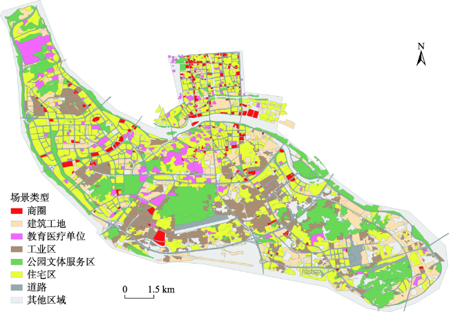
表2 研究区城市场景类型划分说明Tab. 2 Description of urban scene division type division in the experimental area |
| 场景类型 | 说明 |
|---|---|
| 道路 | 高速、主干道、城市道路等主要道路;其他支路属于其邻近的场景 |
| 工业区 | 工业园区、工厂等区域 |
| 教育医疗单位 | 小学、中学、大学和医院 |
| 住宅区 | 住宅楼房及周边绿化区域 |
| 公园文体服务区 | 公园、大型山体公园和体育场等文体服务区域 |
| 建筑工地 | 正在施工的楼房和道路区域 |
| 商圈 | 商业广场和写字楼区域 |
| 其他区域 | 除以上7种类型以外的未具体划分类型的区域 |
表3 空间自相关检验结果Tab. 3 Spatial autocorrelation test |
| 时段 | Moran I指数 | Z得分 | P值 |
|---|---|---|---|
| 8:00 | 0.55 | 9.82 | 0.00 |
| 9:00 | 0.46 | 30.38 | 0.00 |
| 10:00 | 0.84 | 24.45 | 0.00 |
| 11:00 | 0.57 | 48.80 | 0.00 |
| 12:00 | 0.79 | 23.78 | 0.00 |
| 13:00 | 0.82 | 14.51 | 0.00 |
| 14:00 | 0.69 | 22.95 | 0.00 |
| 15:00 | 0.65 | 21.32 | 0.00 |
| 16:00 | 0.82 | 34.66 | 0.00 |
| 17:00 | 0.76 | 21.44 | 0.00 |
| 18:00 | 0.98 | 21.59 | 0.00 |
表4 GWR最优模型构建结果Tab. 4 Model fitting results for GWR |
| 时段 | 预测变量 | R2 | 调整R2 |
|---|---|---|---|
| 8:00 | GL_1500、RES_500、HF_1500、CL_1000、WAT_1000、SEC_1500、PRI_200 | 0.66 | 0.63 |
| 9:00 | CL_1000、PRI_1000、BL_1500、LF_1000、RES_1500、GL_1500、OTH_200、WAT_100、SEC_100 | 0.55 | 0.52 |
| 10:00 | CL_1500、WAT_300、GL_300、SEC_1500、HF_1000、HR_500、LF_500、OTH_200、LR_1000、PRI_1500 | 0.80 | 0.79 |
| 11:00 | CL_1500、SEC_1500、BL_1000、HR_500、LR_300、GL_200 | 0.73 | 0.71 |
| 12:00 | CL_1500、HF_1500、GL_1500、PRI_1500、HR_1500、BL_1000、LF_300、SEC_200、LR_1000 | 0.85 | 0.84 |
| 13:00 | BL_200、OTH_300、LF_1000、CL_1500、LR_1500、RES_1000 | 0.66 | 0.66 |
| 14:00 | RES_1500、HF_500、WAT_1500、CL_500、GL_1500、LF_1500、SEC_1000、LR_500 | 0.68 | 0.79 |
| 15:00 | GL_1500、OTH_1500、WAT_500、HR_1000、PRI_1000、LR_1500、HF_1000 | 0.69 | 0.67 |
| 16:00 | RES_1500、OTH_1000、LF_1500、GL_1500、PRI_1000、LR_200、CL_200 | 0.69 | 0.67 |
| 17:00 | LR_1500、GL_1500、RES_1500、LF_1000、SEC_1500、OTH_1500、PRI_500、CL_1000、WAT_500、HF_300 | 0.85 | 0.85 |
| 18:00 | CL_1500、OTH_1500、RES_1500、HF_200、LF_1500、SEC_500、BL_1500 | 0.92 | 0.92 |
注:GL(绿地面积)、HF(高密度林区面积)、LF(低密度林区面积)、CL(耕地面积)、WAT(水域面积)、BL(扬尘地表面积)、HR(高密度住宅区面积)、LR(低密度住宅区面积)、OTH(其他建筑区面积)、PRI(一级道路长度)、SEC(二级道路长度)、RES(餐饮数量);100、200、300、500、1000、1500分别表示100、200、300、500、1000、1500 m的缓冲区。如GL_1500表示1500 m缓冲区内绿地面积占比。 |
表5 GBDT模型模拟效果Tab. 5 Model fitting results for GBDT |
| 时段 | R2 | RMSE/(μg/m3) | MAE/(μg/m3) |
|---|---|---|---|
| 8:00 | 0.68 | 1.45 | 1.16 |
| 9:00 | 0.80 | 1.61 | 1.20 |
| 10:00 | 0.36 | 4.88 | 3.14 |
| 11:00 | 0.73 | 2.38 | 1.80 |
| 12:00 | 0.80 | 2.23 | 1.66 |
| 13:00 | 0.91 | 1.34 | 1.12 |
| 14:00 | 0.68 | 2.74 | 2.04 |
| 15:00 | 0.88 | 2.60 | 1.99 |
| 16:00 | 0.86 | 4.10 | 3.05 |
| 17:00 | 0.84 | 2.61 | 1.93 |
| 18:00 | 0.99 | 0.73 | 0.57 |
表6 基于GWR-GBDT的PM2.5模拟与场景解析模型模拟效果Tab. 6 Model fitting results of PM2.5 simulation and scene analysis model based on GWR-GBDT |
| 时段 | R2 | RMSE/(μg/m3) | MAE/(μg/m3) | |||||
|---|---|---|---|---|---|---|---|---|
| GWR-GBDT | GWR | GWR-GBDT | GWR | GWR-GBDT | GWR | |||
| 8:00 | 0.89 | 0.66 | 1.45 | 2.55 | 1.16 | 2.00 | ||
| 9:00 | 0.90 | 0.55 | 1.61 | 3.55 | 1.20 | 2.48 | ||
| 10:00 | 0.87 | 0.80 | 4.88 | 6.09 | 3.14 | 3.70 | ||
| 11:00 | 0.92 | 0.73 | 2.38 | 4.54 | 1.80 | 3.18 | ||
| 12:00 | 0.97 | 0.85 | 2.23 | 5.01 | 1.66 | 3.62 | ||
| 13:00 | 0.97 | 0.66 | 1.34 | 4.54 | 1.12 | 3.34 | ||
| 14:00 | 0.90 | 0.68 | 2.74 | 4.87 | 2.04 | 3.62 | ||
| 15:00 | 0.96 | 0.69 | 2.60 | 7.63 | 1.99 | 4.95 | ||
| 16:00 | 0.96 | 0.69 | 4.11 | 11.36 | 3.05 | 8.11 | ||
| 17:00 | 0.98 | 0.85 | 2.61 | 6.52 | 1.93 | 4.64 | ||
| 18:00 | 0.99 | 0.92 | 0.73 | 7.42 | 0.57 | 4.98 | ||
表7 GWR-GBDT模型十折交叉验证结果Tab. 7 10-fold cross validation results of GWR-GBDT model |
| 时段 | R2 | RMSE/(μg/m3) | |||
|---|---|---|---|---|---|
| GWR-GBDT | OLS | GWR-GBDT | OLS | ||
| 8:00 | 0.62 | 0.62 | 2.73 | 2.73 | |
| 9:00 | 0.52 | 0.45 | 3.68 | 3.92 | |
| 10:00 | 0.81 | 0.78 | 5.98 | 6.60 | |
| 11:00 | 0.71 | 0.70 | 4.64 | 4.79 | |
| 12:00 | 0.85 | 0.72 | 5.01 | 7.04 | |
| 13:00 | 0.68 | 0.60 | 4.41 | 5.00 | |
| 14:00 | 0.81 | 0.63 | 3.77 | 5.31 | |
| 15:00 | 0.72 | 0.62 | 7.27 | 8.52 | |
| 16:00 | 0.82 | 0.48 | 8.67 | 14.75 | |
| 17:00 | 0.92 | 0.85 | 4.84 | 6.85 | |
| 18:00 | 0.94 | 0.92 | 6.64 | 7.79 | |
| [1] |
|
| [2] |
生态环境部 生态环境监测规划纲要(2020—2035年)[EB/OL].[2020-06-22]. https://mp.weixin.qq.com/s/NokPfnF3VtT5gSH8693fEA
[Ministry of Ecology and Environment. Outline of ecological environment monitoring planning (2020-2035)[EB/OL] [2020-06-22]. https://mp.weixin.qq.com/s/NokPfnF3VtT5gSH8693fEA
|
| [3] |
|
| [4] |
刘永红, 余志, 黄艳玲, 等. 城市空气污染分布不均匀特征分析[J]. 中国环境监测, 2011, 27(3):93-96.
[
|
| [5] |
|
| [6] |
胡晨霞, 邹滨, 李沈鑫, 等. 城市微环境PM2.5浓度空间分异特征分析[J]. 中国环境科学, 2018, 38(3):910-916.
[
|
| [7] |
|
| [8] |
|
| [9] |
|
| [10] |
|
| [11] |
付宏臣, 孙艳玲, 王斌, 等. 基于AOD数据和GWR模型估算京津冀地区PM2.5浓度[J]. 中国环境科学, 2019, 39(11):4530-4537.
[
|
| [12] |
|
| [13] |
|
| [14] |
|
| [15] |
|
| [16] |
杜震洪, 吴森森, 王中一, 等. 基于地理神经网络加权回归的中国PM2.5浓度空间分布估算方法[J]. 地球信息科学学报, 2020, 22(1):122-135.
[
|
| [17] |
许珊, 邹滨, 胡晨霞. 面向场景的城市PM2.5浓度空间分布精细模拟[J]. 中国环境科学, 2019, 39(11):4570-4579.
[
|
| [18] |
|
| [19] |
|
| [20] |
|
| [21] |
|
| [22] |
|
| [23] |
|
| [24] |
周岩, 谭洪卫, 胡婷莛, 段玉森. 基于移动监测的城市道路PM2.5和PM10浓度分布研究[J]. 环境工程技术学报, 2017, 7(4):433-441.
[
|
| [25] |
宋洁, 周素红, 彭伊侬, 等. 基于移动监测的城市PM2.5污染时空模式研究——以广州市中心区为例[J]. 热带地理, 2020, 40(2):229-242.
[
|
| [26] |
30米空间分辨率全球地表覆盖数据集[DB/OL]. 2020. http://www.globallandcover.com.
[30m spatial resolution global surface coverage data set[DB/OL]. 2020. http://www.globallandcover.com.
|
| [27] |
OpenStreetMap data[DB/OL]. 2021. https://download.geofabrik.de/asia.html
|
| [28] |
李勤勤, 吴爱华, 龚道程, 等. 餐饮源排放PM2.5污染特征研究进展[J]. 环境科学与技术, 2018, 41(8):41-50.
[
|
| [29] |
中国地面气象站逐小时观测资料[DB/OL]. 2021. http://data.cma.cn/data/detail/dataCode/A.0012.0001.html.
[Ho urly observation data of China's surface meteorological stations[DB/OL]. 2021. http://data.cma.cn/data/detail/dataCode/A.0012.0001.html.
|
| [30] |
焦利民, 许刚, 赵素丽, 等. 基于LUR的武汉市PM2.5浓度空间分布模拟[J]. 武汉大学学报·信息科学版, 2015, 40(8):1088-1094.
[
|
| [31] |
夏晓圣, 陈菁菁, 王佳佳, 等. 基于随机森林模型的中国PM2.5浓度影响因素分析[J]. 环境科学, 2020, 41(5):2057-2065.
[
|
| [32] |
王占永, 蔡铭, 彭仲仁, 等. 基于移动观测的路边PM2.5和CO浓度的时空分布[J]. 中国环境科学, 2017, 37(12):4428-4434.
[
|
| [33] |
|
| [34] |
环境空气质量标准:GB3095-2012[S]. 2012.
[Ambient air quality standards:GB3095-2012[S]. 2012. ]
|
| [35] |
蒋燕, 陈波, 鲁绍伟, 等. 北京城市森林PM2.5质量浓度特征及影响因素分析[J]. 生态环境学报, 2016, 25(3):447-457.
[
|
/
| 〈 |
|
〉 |
