
CLAB模型:一种乘客出租出行需求短时预测的深度学习模型
|
周榆欣(1997— ),女,福建长乐人,硕士生,研究方向为时空数据挖掘。E-mail: 531725767@qq.com |
收稿日期: 2022-09-06
修回日期: 2022-10-05
网络出版日期: 2023-03-25
基金资助
国家自然科学基金项目(41471333)
福建省科技计划引导项目(2021H0036)
CLAB Model: A Deep Learning Model for Short-term Prediction of Passenger Rental Travel Demand
Received date: 2022-09-06
Revised date: 2022-10-05
Online published: 2023-03-25
Supported by
National Natural Science Foundation of China(41471333)
Fujian Science and Technology Plan Guidance Project(2021H0036)
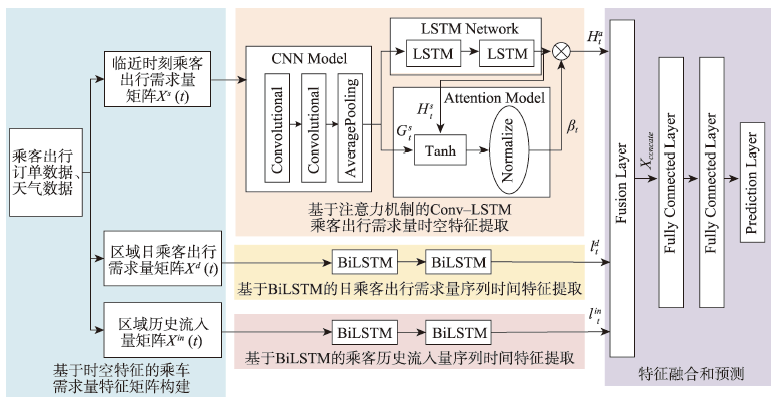
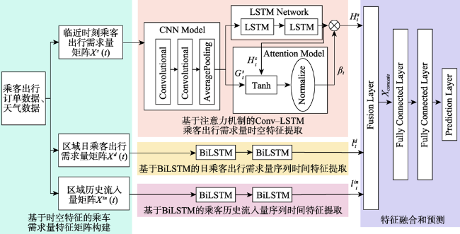
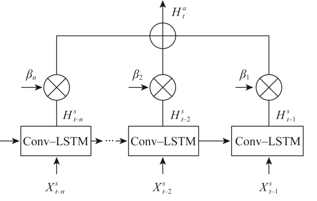
乘客出行需求预测是智能交通系统的组成部分,准确的出行需求预测,对于车辆调度具有重要的意义;然而现有的预测方法无法准确的挖掘其潜在的时空相关性,且大都忽略历史流入量对出行需求的影响。为了进一步挖掘时空大数据中的时空特性及提升模型预测乘客出行需求的精度,本文提出了一种乘客出租出行需求短时预测CLAB(Conv-LSTM Attention BiLSTM)模型。CLAB模型设置了3个模块分别为基于注意力机制的Conv-LSTM模块和2个BiLSTM模块,基于注意力机制的Conv-LSTM模块提取临近时刻乘客出行需求量中的空间特征和短时时间特征,其中注意力机制能自动分配不同的权重来判别不同时间的需求量序列重要性;为了探索长期时间特征,用2个BiLSTM模块来提取历史流入量序列时间特征和日乘客需求量序列的时间特征。采用厦门岛的网约车和巡游车的订单数据进行实验,结果表明:① CLAB模型更适用于使用30 min历史数据预测未来5 min短时乘客出行需求;② 与基准预测模型相比,CLAB模型的整体的效果误差更低,具有更好的预测效果,CLAB模型比CNN-LSTM、LSTM、BiLSTM、CNN和Conv-LSTM的平均绝对误差(MAE)分别降低了33.179%、33.153%、33.204%、5.401%和5.914%,均方根误差(RMSE)分别降低了34.389%、34.423%、34.524%、6.772%和6.669%;③ 同时发现CLAB模型在规律性较高的工作日预测效果优于非工作日,且工作日早高峰预测效果最佳。
周榆欣 , 邬群勇 . CLAB模型:一种乘客出租出行需求短时预测的深度学习模型[J]. 地球信息科学学报, 2023 , 25(1) : 77 -89 . DOI: 10.12082/dqxxkx.2023.220662
Passenger travel demand prediction is an integral part of intelligent transportation systems, and accurate travel demand prediction is of great significance for vehicle scheduling. However, existing prediction methods are unable to accurately explore its potential spatiotemporal correlation and mostly ignore the impact of historical inflow on travel demand. In order to further exploit the spatiotemporal characteristics of spatiotemporal big data and improve the accuracy of the model in predicting passenger travel demand, this paper proposes a Conv-LSTM Attention BiLSTM (CLAB) model for short-time prediction of passenger rental travel demand. The attention-based Conv-LSTM module extracts spatial features and short-term temporal features of passenger travel demand at the near moment, where the attention mechanism automatically assigns different weights to discriminate the importance of demand sequences at different times. To explore long-term temporal features, two BiLSTM modules are used to extract temporal features of historical inflow sequences and temporal features of daily passenger temporal features of the demand series. Experiments are conducted using the order data of online and cruising taxis on Xiamen Island, and the results show that: (1) the CLAB model is more suitable for predicting the future 5-min short-time passenger travel demand using 30-min historical data; (2) the overall effect error of the CLAB model is lower and has better prediction results compared with the benchmark prediction model. The CLAB model is more effective than the CNN-LSTM, LSTM, BiLSTM, CNN, and Conv-LSTM by 33.179%, 33.153%, 33.204%, 5.401%, and 5.914% in mean absolute error (MAE) and 34.389%, 34.423%, 34.524%, 6.772%, and 6.669% in Root Mean Square Error (RMSE), respectively; (3) the CLAB model performs better for weekday prediction with higher regularity than non-working day prediction, with best prediction for weekday morning peaks.
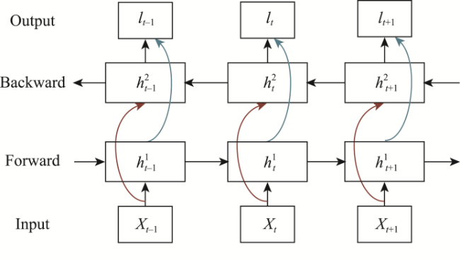
图3 双向长短时记忆神经网络结构示意注: Xt-1、Xt、Xt+1为不同时刻的输入(Input); h1t-1、h1t、h1t+1为不同时刻正向(Forward)LSTM的输出; h2t-1、h2t、h2t+1为不同时刻反向(Backward)LSTM的输出;lt-1、lt、lt+1对应不同时刻正向LSTM和反向LSTM输出拼接得到输出向量(Output)。 Fig. 3 Schematic diagram of the structure of a bidirectional long-and short-term memory neural network |
表1 不同批量大小的实验结果Tab. 1 Experimental results for different batchsizes |
| batch_size | MAE | RMSE |
|---|---|---|
| 16 | 1.756 | 2.575 |
| 32 | 1.737 | 2.564 |
| 60 | 1.734 | 2.547 |
| 128 | 1.742 | 2.589 |
表2 不同组件层数的实验结果Tab. 2 Experimental results for different component layers |
| 组件层数 | MAE | RMSE |
|---|---|---|
| 1 | 1.750 | 2.571 |
| 2 | 1.734 | 2.547 |
| 3 | 1.747 | 2.571 |
| 4 | 1.750 | 2.589 |
表3 CLAB模型不同时间片划分对比实验Tab. 3 CLAB model different time slice division comparison experiment |
| 时间/min | 30 min | 60 min | ||||
|---|---|---|---|---|---|---|
| MAE | RMSE | MAE | RMSE | |||
| 5 | 1.734 | 2.547 | 1.753 | 2.581 | ||
| 10 | 2.664 | 4.122 | 2.714 | 4.158 | ||
| 15 | 3.660 | 5.741 | 3.667 | 5.671 | ||
表4 不同方法在预测时长为5 min下的性能对比Tab. 4 Comparison of the performance of different methods at a prediction duration of 5 min |
| 模型 | MAE | RMSE |
|---|---|---|
| CNN-LSTM | 2.595 | 3.882 |
| LSTM | 2.594 | 3.884 |
| BiLSTM | 2.596 | 3.890 |
| CNN | 1.833 | 2.732 |
| ConvLSTM | 1.843 | 2.729 |
| CLAB | 1.734 | 2.547 |
表5 CLAB模型在预测时长为5 min下消融实验Tab. 5 CLAB model ablation experiment at a predicted duration of 5 min |
| 模型 | 加入其它影响因素 | 无其它影响因素 | ||||
|---|---|---|---|---|---|---|
| MAE | RMSE | MAE | RMSE | |||
| A去掉注意力机制 | 1.735 | 2.587 | 1.740 | 2.569 | ||
| B去掉历史流入量 | 1.744 | 2.587 | 1.761 | 2.624 | ||
| C去掉日乘客需求量 | 1.742 | 2.558 | 1.766 | 2.618 | ||
| D 去掉历史流入量和日乘客需求量 | 1.752 | 2.596 | 1.740 | 2.582 | ||
| E 去掉流入量、日乘客需求量和注意力机制 | 1.738 | 2.579 | 1.748 | 2.592 | ||
| CLAB | 1.734 | 2.547 | 1.739 | 2.565 | ||
表6 CLAB模型在工作日和非工作日高峰期性能对比Tab. 6 Comparison of CLAB model performance during peak weekday and non-weekday periods |
| MAE | RMSE | ||||||||
|---|---|---|---|---|---|---|---|---|---|
| 全天 | 早高峰 | 午高峰 | 晚高峰 | 全天 | 早高峰 | 午高峰 | 晚高峰 | ||
| 工作日 | 1.780 | 1.444 | 1.879 | 2.138 | 2.544 | 1.946 | 2.548 | 2.910 | |
| 非工作日 | 1.688 | 2.158 | 1.810 | 2.164 | 2.550 | 2.862 | 2.505 | 3.230 | |
| [1] |
|
| [2] |
|
| [3] |
|
| [4] |
|
| [5] |
|
| [6] |
|
| [7] |
|
| [8] |
|
| [9] |
|
| [10] |
|
| [11] |
|
| [12] |
|
| [13] |
|
| [14] |
|
| [15] |
|
| [16] |
|
| [17] |
|
| [18] |
|
| [19] |
|
| [20] |
|
| [21] |
|
| [22] |
|
| [23] |
|
| [24] |
|
| [25] |
路民超, 李建波, 逄俊杰, 等. 面向出租车需求预测的多因素时空图卷积网络[J]. 计算机工程与应用, 2020, 56(24):266-273.
[
|
| [26] |
|
| [27] |
程静, 刘家骏, 高勇. 基于时间序列聚类方法分析北京出租车出行量的时空特征[J]. 地球信息科学学报, 2016, 18(9):1227-1239.
[
|
| [28] |
厦门市统计局. 厦门经济特区年鉴[M]. 北京: 中国统计出版社, 2021.
[Bureau of Statistics of Xiamen. Yearbook of Xiamen special economic zone[M]. Beijing: China Statistics Press, 2021. ]
|
| [29] |
|
| [30] |
|
| [31] |
|
| [32] |
|
| [33] |
张维, 袁绍欣, 陶建军, 等. 基于多元因素的Bi-LSTM高速公路交通流预测[J]. 计算机系统应用, 2021, 30(6):184-190.
[
|
/
| 〈 |
|
〉 |
