
面向高光谱影像小样本分类的全局-局部特征自适应融合方法
|
左溪冰(1996— ),男,湖南长沙人,博士生,主要从事遥感图像智能解译研究。E-mail: zuoxibing1015@163.com |
收稿日期: 2023-02-11
修回日期: 2023-03-12
网络出版日期: 2023-07-14
基金资助
河南省自然科学基金项目(222300420387)
Global-local Feature Adaptive Fusion Method for Small Sample Classification of Hyperspectral Images
Received date: 2023-02-11
Revised date: 2023-03-12
Online published: 2023-07-14
Supported by
Natural Science Foundation of Henan Province(222300420387)
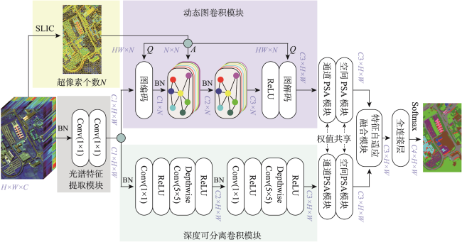
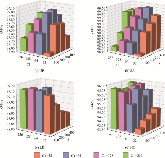
高光谱影像标记样本的获取通常是一项费时费力的工作,如何在小样本条件下提高影像的分类精度是高光谱影像分类领域面临的难题之一。现有的高光谱影像分类方法对影像的多尺度信息挖掘不够充分,导致在小样本条件下的分类精度较差。针对此问题,本文设计了一种面向高光谱影像小样本分类的全局特征与局部特征自适应融合方法。该方法基于动态图卷积网络和深度可分离卷积网络,分别从全局尺度和局部尺度挖掘影像的潜在信息,实现了标记样本的有效利用。进一步引入极化自注意力机制,在减少信息损失的同时提升网络的特征表达,并采用特征自适应融合机制对全局特征和局部特征进行自适应融合。为验证本文方法的有效性,在University of Pavia、Salinas、WHU-Hi-LongKou和WHU-Hi-HanChuan4组高光谱影像基准数据集上开展分类试验。试验结果表明,与传统分类器和先进的深度学习模型相比,本文方法兼顾执行效率和分类精度,在小样本条件下能够取得更为优异的分类表现。在4组数据集上的总体分类精度分别为99.01%、99.42%、99.18%和95.84%,平均分类精度分别为99.31%、99.65%、98.89%和95.49%,Kappa系数分别为98.69%、99.35%、98.93%和95.14%。本文方法对应的代码开源于 https://github.com/IceStreams/GLFAF。
左溪冰 , 刘智 , 金飞 , 林雨准 , 王淑香 , 刘潇 , 李美霖 . 面向高光谱影像小样本分类的全局-局部特征自适应融合方法[J]. 地球信息科学学报, 2023 , 25(8) : 1699 -1716 . DOI: 10.12082/dqxxkx.2023.230058
Acquisition of labeled samples for hyperspectral image classification is usually a time- and labor- consuming task. How to effectively improve the classification accuracy using a small number of samples is one of the challenges in the field of hyperspectral image classification. Most of existing classification methods for hyperspectral images lack sufficient multi-scale information mining, which leads to unsatisfactory classification performance due to small sample numbers. To address the aforementioned issue, this paper designed an adaptive fusion method by integrating global and local features for hyperspectral image classification with small sample numbers. Based on the dynamic graph convolutional network and the depth wise separable convolutional network, a two-branch network structure was constructed to mine the potential information of hyperspectral images from the global and local scales, which realizes the effective usage of labeled samples. Furthermore, the polarization self-attention mechanism was introduced to further improve the expression of intermediate features in the network while cutting down the loss of feature information, and the adaptive feature fusion mechanism was adopted to carry out adaptive fusion of global and local features. Finally, the fusion features flow into the full-connection layer and are manipulated by softmax to obtain prediction labels for each pixel of the hyperspectral image. In order to verify the effectiveness of the proposed method, classification experiments were carried out on four hyperspectral image benchmark data sets including University of Pavia, Salinas, WHU-Hi-LongKou, and WHU-Hi-HanChuan. We discussed and analyzed the influence of model parameters and different modules on the classification accuracy. Subsequently, a comprehensive comparison with seven existing advanced classification methods was conducted in terms of classification visualization, classification accuracy, number of labeled samples, and execution efficiency. The experimental results show that the dynamic graph convolutional network, depth wise separable convolutional network, the polarization self-attention mechanism, and the adaptive feature fusion mechanism all contributed to the improvement of hyperspectral image classification accuracy. In addition, compared with traditional classifiers and advanced deep learning models, the proposed method considered both execution efficiency and classification accuracy, and can achieve better classification performance under the condition of small sample numbers. Specifically, on these four data sets (i.e., University of Pavia, Salinas, WHU-Hi-LongKou and WHU-Hi-HanChuan). The overall classification accuracy was 99.01%, 99.42%, 99.18% and 95.84%, respectively; the average classification accuracy was 99.31%, 99.65%, 98.89% and 95.49%, respectively; and the Kappa coefficient was 98.69%, 99.35%, 98.93% and 95.14%, respectively. The corresponding source code will be available at https://github.com/IceStreams/GLFAF.
表1 GLFAF的部分网络结构参数Tab. 1 The partial network structure parameters of GLFAF |
| 模块 | 网络层 | 输入特征 | 输出特征 | 滤波器尺寸 |
|---|---|---|---|---|
| SFE | Conv1_1 | C×H×W | C1×H×W | 1×1 (C1) |
| Conv1_2 | C1×H×W | C1×H×W | 1×1 (C1) | |
| DGC | 图编码层 | C1×H×W | C1×N | HW×N |
| W1 | C1×N | C2×N | C1×C2 | |
| W2 | C2×N | C3×N | C2×C3 | |
| 图解码层 | C3×N | C3×H×W | HW×N | |
| DSC | Conv2_1 | C1×H×W | C2×H×W | 1×1 (C2) |
| Conv2_2 | C2×H×W | C2×H×W | 5×5 (C2) | |
| Conv2_3 | C2×H×W | C3×H×W | 1×1 (C3) | |
| Conv2_4 | C3×H×W | C3×H×W | 5×5 (C3) | |
| 通道PSA | Conv3_1 | CC3×H×W | C3/2×H×W | 1×1 (C3/2) |
| Conv3_2 | C3×H×W | 1×H×W | 1×1 (1) | |
| Conv3_3 | C3/2×1×1 | C3×1×1 | 1×1 (C3) | |
| 空间PSA | Conv4_1 | C3×H×W | C3/2×H×W | 1×1 (C3/2) |
| Conv4_2 | C3×H×W | C3/2×H×W | 1×1 (C3/2) | |
| AFF | Conv5_1 | C3×1×1 | C3×1×1 | 1×1 (C3) |
| Conv5_2 | C3×1×1 | C3×1×1 | 1×1 (C3) | |
| Conv5_3 | C3×H×W | C3×H×W | 1×1 (C3) | |
| Conv5_4 | C3×H×W | C3×H×W | 1×1 (C3) | |
| 全连接层 | C3×H×W | C4×H×W | C3×C4 | |
表2 UP数据集地物类别与样本数量Tab. 2 Category of ground objects and sample number of UP data set (个) |
| 类别序号 | 类别名称 | 训练样本 | 验证样本 | 测试样本 |
|---|---|---|---|---|
| 1 | 沥青路面 | 40 | 10 | 6 631 |
| 2 | 草地 | 40 | 10 | 18 649 |
| 3 | 砂砾 | 40 | 10 | 2 099 |
| 4 | 树木 | 40 | 10 | 3 064 |
| 5 | 金属板 | 40 | 10 | 1 345 |
| 6 | 裸地 | 40 | 10 | 5 029 |
| 7 | 沥青屋顶 | 40 | 10 | 1 330 |
| 8 | 砖块 | 40 | 10 | 3 682 |
| 9 | 阴影 | 40 | 10 | 947 |
| 总计 | 360 | 90 | 42 776 | |
表3 SA数据集地物类别与样本数量Tab. 3 Category of ground objects and sample number of SA data set (个) |
| 类别序号 | 类别名称 | 训练样本 | 验证样本 | 测试样本 |
|---|---|---|---|---|
| 1 | 花椰菜-绿地-野草-1 | 40 | 10 | 2 009 |
| 2 | 花椰菜-绿地-野草-2 | 40 | 10 | 3 726 |
| 3 | 休耕地 | 40 | 10 | 1 976 |
| 4 | 休耕地-荒地-犁地 | 40 | 10 | 1 394 |
| 5 | 休耕地-平地 | 40 | 10 | 2 678 |
| 6 | 茬地 | 40 | 10 | 3 959 |
| 7 | 芹菜 | 40 | 10 | 3 579 |
| 8 | 葡萄-未培地 | 40 | 10 | 11 271 |
| 9 | 土壤-葡萄园-开发地 | 40 | 10 | 6 203 |
| 10 | 谷地-衰败地-绿地-野草 | 40 | 10 | 3 278 |
| 11 | 生菜-莴苣-4周 | 40 | 10 | 1 068 |
| 12 | 生菜-莴苣-5周 | 40 | 10 | 1 927 |
| 13 | 生菜-莴苣-6周 | 40 | 10 | 916 |
| 14 | 生菜-莴苣-7周 | 40 | 10 | 1 070 |
| 15 | 葡萄园-未培地 | 40 | 10 | 7 268 |
| 16 | 葡萄园-垂直棚架 | 40 | 10 | 1 807 |
| 总计 | 640 | 160 | 54 129 | |
表4 LK数据集地物类别与样本数量Tab. 4 Category of ground objects and sample number of LK data set (个) |
| 类别序号 | 类别名称 | 训练样本 | 验证样本 | 测试样本 |
|---|---|---|---|---|
| 1 | 玉米 | 40 | 10 | 34 511 |
| 2 | 棉花 | 40 | 10 | 8 374 |
| 3 | 芝麻 | 40 | 10 | 3 031 |
| 4 | 阔叶大豆 | 40 | 10 | 63 212 |
| 5 | 窄叶大豆 | 40 | 10 | 4 151 |
| 6 | 大米 | 40 | 10 | 11 854 |
| 7 | 水 | 40 | 10 | 67 056 |
| 8 | 道路和房屋 | 40 | 10 | 7 124 |
| 9 | 混合杂草 | 40 | 10 | 5 229 |
| 总计 | 360 | 90 | 204 542 | |
表5 HC数据集地物类别与样本数量Tab. 5 Category of ground objects and sample number of HC data set (个) |
| 类别序号 | 类别名称 | 训练样本 | 验证样本 | 测试样本 |
|---|---|---|---|---|
| 1 | 草莓 | 40 | 10 | 44 735 |
| 2 | 豇豆 | 40 | 10 | 22 753 |
| 3 | 大豆 | 40 | 10 | 10 287 |
| 4 | 高粱 | 40 | 10 | 5 353 |
| 5 | 空心菜 | 40 | 10 | 1 200 |
| 6 | 西瓜 | 40 | 10 | 4 533 |
| 7 | 绿色植被 | 40 | 10 | 5 903 |
| 8 | 树 | 40 | 10 | 17 978 |
| 9 | 草地 | 40 | 10 | 9 469 |
| 10 | 红色屋顶 | 40 | 10 | 10 516 |
| 11 | 灰色屋顶 | 40 | 10 | 16 911 |
| 12 | 塑料 | 40 | 10 | 3 679 |
| 13 | 裸土 | 40 | 10 | 9 116 |
| 14 | 道路 | 40 | 10 | 18 560 |
| 15 | 明亮物体 | 40 | 10 | 1 136 |
| 16 | 水 | 40 | 10 | 75 401 |
| 总计 | 640 | 160 | 257 530 | |
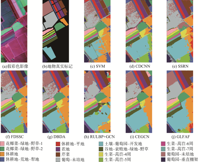
图6 UP数据集上不同分类方法的分类结果Fig. 6 The classification result of different classification methods on the UP data set |
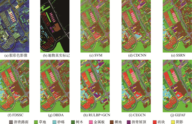
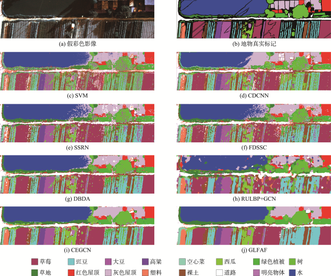
图7 SA数据集上不同分类方法的分类结果Fig. 7 The classification result of different classification methods on the SA data set |
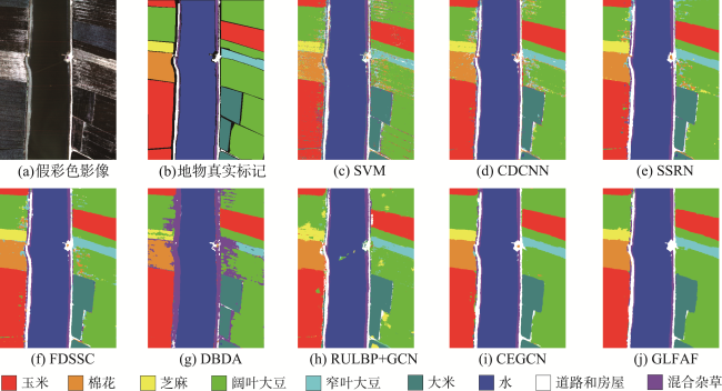
图8 LK数据集上不同分类方法的分类结果Fig. 8 The classification result of different classification methods on the LK data set |
表6 UP数据集上不同分类方法的分类结果Tab. 6 Classification results of different classification methods on the UP dataset |
| 类别序号 | SVM | CDCNN | SSRN | FDSSC | DBDA | RULBP+GCN | CEGCN | GLFAF |
|---|---|---|---|---|---|---|---|---|
| 1 | 91.92 | 94.82 | 99.28 | 99.12 | 99.02 | 97.33 | 99.06 | 99.10 |
| 2 | 94.25 | 97.23 | 99.25 | 98.93 | 99.21 | 99.35 | 96.54 | 98.76 |
| 3 | 66.97 | 71.53 | 83.40 | 81.75 | 89.06 | 85.67 | 98.79 | 99.96 |
| 4 | 72.40 | 89.24 | 95.91 | 93.76 | 91.28 | 92.07 | 97.67 | 97.62 |
| 5 | 95.68 | 99.46 | 100.00 | 99.99 | 99.89 | 99.98 | 100.00 | 100.00 |
| 6 | 61.17 | 64.76 | 89.05 | 94.13 | 91.61 | 92.99 | 99.65 | 99.79 |
| 7 | 58.70 | 69.60 | 91.78 | 95.18 | 98.24 | 80.78 | 99.95 | 99.90 |
| 8 | 82.78 | 86.23 | 91.36 | 87.63 | 92.15 | 94.06 | 96.96 | 98.72 |
| 9 | 99.96 | 89.05 | 99.66 | 99.29 | 98.88 | 90.64 | 99.92 | 99.93 |
| OA/% | 81.70 | 86.15 | 95.55 | 95.58 | 96.05 | 95.48 | 97.81 | 99.01 |
| AA/% | 80.43 | 84.66 | 94.41 | 94.42 | 95.48 | 92.54 | 98.73 | 99.31 |
| Kappa/% | 76.64 | 82.24 | 94.17 | 94.20 | 94.83 | 94.08 | 97.16 | 98.69 |
注:加粗数值表示表格中每一行的最佳值。 |
表7 SA数据集上不同分类方法的分类结果Tab. 7 Classification results of different classification methods on the SA dataset |
| 类别序号 | SVM | CDCNN | SSRN | FDSSC | DBDA | RULBP+GCN | CEGCN | GLFAF |
|---|---|---|---|---|---|---|---|---|
| 1 | 99.88 | 99.49 | 98.35 | 100.00 | 100.00 | 99.83 | 100.00 | 100.00 |
| 2 | 98.94 | 99.05 | 99.29 | 99.74 | 99.97 | 99.97 | 100.00 | 100.00 |
| 3 | 94.02 | 95.15 | 98.91 | 98.94 | 98.72 | 98.83 | 100.00 | 100.00 |
| 4 | 97.79 | 99.07 | 98.94 | 99.01 | 99.27 | 94.61 | 99.96 | 99.91 |
| 5 | 98.71 | 97.66 | 99.44 | 99.49 | 99.12 | 99.40 | 99.47 | 99.70 |
| 6 | 99.46 | 98.82 | 99.94 | 99.97 | 100.00 | 98.79 | 99.99 | 99.95 |
| 7 | 98.84 | 99.55 | 99.94 | 99.81 | 99.86 | 99.93 | 99.94 | 99.96 |
| 8 | 80.36 | 80.49 | 88.83 | 90.18 | 91.83 | 94.03 | 90.09 | 98.52 |
| 9 | 99.11 | 99.56 | 99.80 | 99.66 | 99.28 | 99.89 | 100.00 | 100.00 |
| 10 | 86.05 | 87.87 | 96.61 | 97.20 | 95.79 | 99.40 | 96.77 | 97.83 |
| 11 | 83.83 | 85.39 | 97.23 | 96.97 | 96.32 | 97.86 | 99.78 | 99.93 |
| 12 | 95.99 | 98.49 | 99.33 | 99.26 | 99.38 | 99.62 | 100.00 | 99.94 |
| 13 | 95.77 | 95.91 | 97.94 | 99.64 | 99.84 | 98.76 | 99.95 | 99.91 |
| 14 | 90.29 | 91.41 | 90.84 | 95.64 | 96.66 | 96.05 | 99.58 | 99.52 |
| 15 | 64.61 | 68.94 | 72.01 | 80.99 | 78.95 | 86.45 | 92.75 | 99.23 |
| 16 | 97.19 | 97.91 | 99.37 | 99.47 | 99.59 | 94.45 | 99.51 | 99.93 |
| OA/% | 88.44 | 89.00 | 91.60 | 94.64 | 94.22 | 96.10 | 96.71 | 99.42 |
| AA/% | 92.55 | 93.42 | 96.05 | 97.25 | 97.16 | 97.37 | 98.61 | 99.65 |
| Kappa/% | 87.17 | 87.78 | 90.67 | 94.04 | 93.58 | 95.66 | 96.34 | 99.35 |
注:加粗数值表示表格中每一行的最佳值。 |
表8 LK数据集上不同分类方法的分类结果Tab. 8 Classification results of different classification methods on the LK dataset |
| 类别序号 | SVM | CDCNN | SSRN | FDSSC | DBDA | RULBP+GCN | CEGCN | GLFAF |
|---|---|---|---|---|---|---|---|---|
| 1 | 96.69 | 98.53 | 99.50 | 99.72 | 99.73 | 98.97 | 99.89 | 99.90 |
| 2 | 64.75 | 79.04 | 90.67 | 84.95 | 91.10 | 99.18 | 99.53 | 99.83 |
| 3 | 45.71 | 68.04 | 90.93 | 93.05 | 91.18 | 48.25 | 99.72 | 99.60 |
| 4 | 97.72 | 98.68 | 99.58 | 99.63 | 99.62 | 99.16 | 97.91 | 98.33 |
| 5 | 52.18 | 64.21 | 75.98 | 83.51 | 79.43 | 66.26 | 99.27 | 99.50 |
| 6 | 95.80 | 98.95 | 99.34 | 99.65 | 99.56 | 97.66 | 99.69 | 99.62 |
| 7 | 99.96 | 99.72 | 99.94 | 99.97 | 99.98 | 99.97 | 99.93 | 99.90 |
| 8 | 88.11 | 88.64 | 91.67 | 95.37 | 93.84 | 91.65 | 96.62 | 95.91 |
| 9 | 70.72 | 77.94 | 88.55 | 87.16 | 81.01 | 88.06 | 96.92 | 97.43 |
| OA/% | 91.89 | 95.08 | 97.73 | 98.03 | 97.24 | 96.08 | 99.06 | 99.18 |
| AA/% | 79.07 | 85.97 | 92.91 | 93.67 | 92.58 | 87.68 | 98.83 | 98.89 |
| Kappa/% | 89.53 | 93.61 | 97.03 | 97.42 | 96.40 | 94.91 | 98.77 | 98.93 |
注:加粗数值表示表格中每一行的最佳值。 |
表9 HC数据集上不同分类方法的分类结果Tab. 9 Classification results of different classification methods on the HC dataset |
| 类别序号 | SVM | CDCNN | SSRN | FDSSC | DBDA | RULBP+GCN | CEGCN | GLFAF |
|---|---|---|---|---|---|---|---|---|
| 1 | 92.04 | 94.04 | 89.46 | 93.95 | 95.43 | 90.86 | 95.29 | 95.90 |
| 2 | 69.61 | 83.37 | 89.62 | 92.66 | 95.71 | 93.25 | 81.64 | 90.38 |
| 3 | 53.57 | 68.17 | 66.58 | 71.47 | 77.80 | 83.24 | 95.07 | 96.76 |
| 4 | 78.56 | 91.88 | 82.13 | 91.81 | 91.95 | 76.54 | 98.19 | 98.89 |
| 5 | 13.57 | 38.25 | 51.39 | 43.72 | 47.60 | 45.03 | 99.64 | 99.69 |
| 6 | 20.26 | 26.37 | 46.21 | 51.09 | 65.04 | 55.41 | 90.29 | 95.32 |
| 7 | 54.03 | 60.10 | 57.61 | 65.82 | 70.18 | 63.74 | 96.34 | 98.66 |
| 8 | 68.75 | 79.02 | 91.09 | 91.46 | 95.10 | 89.96 | 80.17 | 90.32 |
| 9 | 56.32 | 59.80 | 71.32 | 76.87 | 80.78 | 59.00 | 89.89 | 93.25 |
| 10 | 83.88 | 96.46 | 87.52 | 91.50 | 98.45 | 62.53 | 97.70 | 97.26 |
| 11 | 56.75 | 69.41 | 69.46 | 74.19 | 87.37 | 58.22 | 98.29 | 98.13 |
| 12 | 25.70 | 42.06 | 59.28 | 57.14 | 65.11 | 62.03 | 94.74 | 99.10 |
| 13 | 38.46 | 42.49 | 44.24 | 51.28 | 59.73 | 50.39 | 80.95 | 87.47 |
| 14 | 77.72 | 81.05 | 77.01 | 81.30 | 90.57 | 83.98 | 88.99 | 93.25 |
| 15 | 39.87 | 55.13 | 43.47 | 65.85 | 81.22 | 31.61 | 93.58 | 94.19 |
| 16 | 99.89 | 98.55 | 97.97 | 99.68 | 99.93 | 98.03 | 98.27 | 99.30 |
| OA/% | 71.02 | 77.87 | 79.72 | 84.98 | 89.98 | 79.78 | 93.03 | 95.84 |
| AA/% | 58.06 | 67.89 | 70.27 | 74.99 | 81.37 | 69.99 | 92.44 | 95.49 |
| Kappa/% | 66.88 | 74.56 | 76.50 | 82.62 | 88.35 | 76.81 | 91.87 | 95.14 |
注:加粗数值表示表格中每一行的最佳值。 |
表10 4组数据集上的消融试验结果Tab. 10 Results of ablation experiments on four data sets |
| 试验组 | 网络模块 | 数据集 | |||||||
|---|---|---|---|---|---|---|---|---|---|
| SFE | DGC | DSC | PSA | AFF | UP | SA | LK | HC | |
| A | √ | √ | √ | √ | √ | 99.01 | 99.42 | 99.18 | 95.84 |
| B | × | √ | √ | √ | √ | 98.47 | 98.07 | 98.52 | 95.08 |
| C | √ | × | √ | √ | √ | 97.04 | 96.78 | 98.99 | 94.69 |
| D | √ | √ | × | √ | √ | 94.59 | 98.96 | 98.35 | 94.91 |
| E | √ | √ | √ | × | √ | 98.81 | 99.38 | 99.01 | 95.05 |
| F | √ | √ | √ | √ | × | 98.70 | 98.86 | 99.03 | 95.38 |
表11 不同分类方法在4组数据集上的执行效率对比Tab. 11 Comparison of execution efficiency of different classification methods on four data sets |
| 数据集 | 衡量指标 | CDCNN | SSRN | FDSSC | DBDA | RULBP+GCN | CEGCN | GLFAF |
|---|---|---|---|---|---|---|---|---|
| UP | Params/M | 0.63 | 0.22 | 0.65 | 0.20 | 1.58×10⁻³ | 0.15 | 0.18 |
| FLOPs/G | 0.76 | 19.32 | 11.10 | 85.01 | 1.15×10⁻⁵ | 126.99 | 65.29 | |
| Training/s | 0.15 | 1.84 | 2.36 | 0.15 | 0.66 | 0.22 | 0.36 | |
| Testing/s | 0.70 | 4.83 | 9.90 | 9.58 | 1.38 | 1.29 | 1.31 | |
| SA | Params/M | 1.08 | 0.37 | 1.25 | 0.39 | 3.54×10⁻³ | 0.17 | 0.18 |
| FLOPs/G | 0.37 | 10.02 | 5.69 | 3.47 | 2.55×10⁻⁵ | 36.61 | 20.10 | |
| Training/s | 0.25 | 3.43 | 4.31 | 0.40 | 0.17 | 0.11 | 0.20 | |
| Testing/s | 1.17 | 11.84 | 22.94 | 23.83 | 0.99 | 0.91 | 0.95 | |
| LK | Params/M | 1.38 | 0.47 | 1.64 | 0.51 | 1.58×10⁻³ | 0.17 | 0.19 |
| FLOPs/G | 4.69 | 128.05 | 72.53 | 44.28 | 1.15×10⁻⁵ | 139.22 | 85.57 | |
| Training/s | 0.16 | 2.00 | 2.52 | 0.30 | 0.69 | 0.24 | 0.41 | |
| Testing/s | 5.80 | 88.16 | 119.75 | 121.80 | 2.47 | 2.52 | 2.55 | |
| HC | Params/M | 1.40 | 0.48 | 1.67 | 0.52 | 1.81×10⁻³ | 0.18 | 0.19 |
| FLOPs/G | 3.58 | 97.61 | 55.28 | 33.75 | 0.13×10⁻⁵ | 393.40 | 213.08 | |
| Training/s | 0.26 | 3.54 | 1.86 | 1.05 | 0.47 | 0.32 | 0.29 | |
| Testing/s | 27.17 | 111.60 | 46.43 | 61.14 | 1.93 | 11.61 | 12.65 |
| [1] |
余旭初, 冯伍法, 杨国鹏, 等. 高光谱影像分析与应用[M]. 北京: 科学出版社, 2013.
[
|
| [2] |
|
| [3] |
|
| [4] |
|
| [5] |
|
| [6] |
|
| [7] |
|
| [8] |
|
| [9] |
|
| [10] |
李玉, 李奕燃, 王光辉, 等. 基于加权指数函数模型的高光谱图像分类方法[J]. 地球信息科学学报, 2020, 22(8):1642-1653.
[
|
| [11] |
杜培军, 夏俊士, 薛朝辉, 等. 高光谱遥感影像分类研究进展[J]. 遥感学报, 2016, 20(2):236-256.
[
|
| [12] |
马晓瑞. 基于深度学习的高光谱影像分类方法研究[D]. 大连: 大连理工大学, 2017.
[
|
| [13] |
张号逵, 李映, 姜晔楠. 深度学习在高光谱图像分类领域的研究现状与展望[J]. 自动化学报, 2018, 44(6):961-977.
[
|
| [14] |
余岸竹, 刘冰, 邢志鹏, 等. 面向高光谱影像分类的显著性特征提取方法[J]. 测绘学报, 2019, 48(8):985-995.
[
|
| [15] |
|
| [16] |
|
| [17] |
|
| [18] |
|
| [19] |
|
| [20] |
|
| [21] |
|
| [22] |
|
| [23] |
左溪冰, 刘冰, 余旭初, 等. 高光谱影像小样本分类的图卷积网络方法[J]. 测绘学报, 2021, 50(10):1358-1369.
[
|
| [24] |
|
| [25] |
|
| [26] |
|
| [27] |
|
| [28] |
|
| [29] |
|
| [30] |
|
| [31] |
刘冰, 余旭初, 张鹏强, 等. 联合空-谱信息的高光谱影像深度三维卷积网络分类[J]. 测绘学报, 2019, 48(1):53-63.
[
|
| [32] |
|
| [33] |
|
| [34] |
|
| [35] |
|
/
| 〈 |
|
〉 |