
基于多元时间序列动态图神经网络的交通速度预测
作者贡献:Author Contributions
练培格和李英冰参与实验设计;练培格、刘波、冯晓珂完成实验操作;练培格、李英冰、刘波、冯晓珂参与论文的写作和修改。所有作者均阅读并同意最终稿件的提交。
The study was designed by LIAN Peige and LI Yingbing. The experiment operation was completed by LIAN Peige LIU Bo and FENG Xiaoke. The manuscript was drafted and revised by LIAN Peige, LI Yingbing, LIU Bo and FENG Xiaoke. All the authors have read the last version of paper and consented for submission.
|
练培格(2000— ),女,河南平顶山人,硕士生,主要从交通预测研究。E-mail: lianpeige@163.com |
收稿日期: 2024-11-17
修回日期: 2025-01-06
网络出版日期: 2025-03-06
基金资助
国家重点研发计划项目(2018YFC0807000)
Traffic Speed Prediction Using Multivariate Time Series Dynamic Graph Neural Network
Received date: 2024-11-17
Revised date: 2025-01-06
Online published: 2025-03-06
Supported by
National Key Research and Development Program of China(2018YFC0807000)
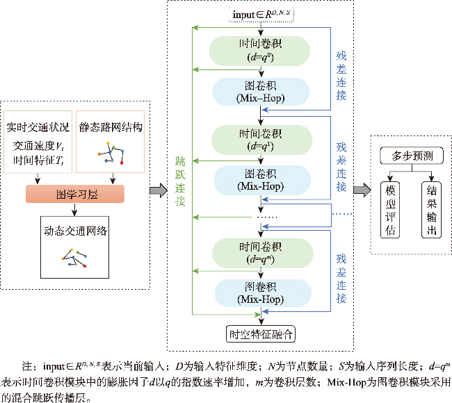
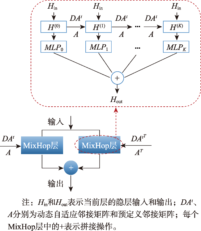
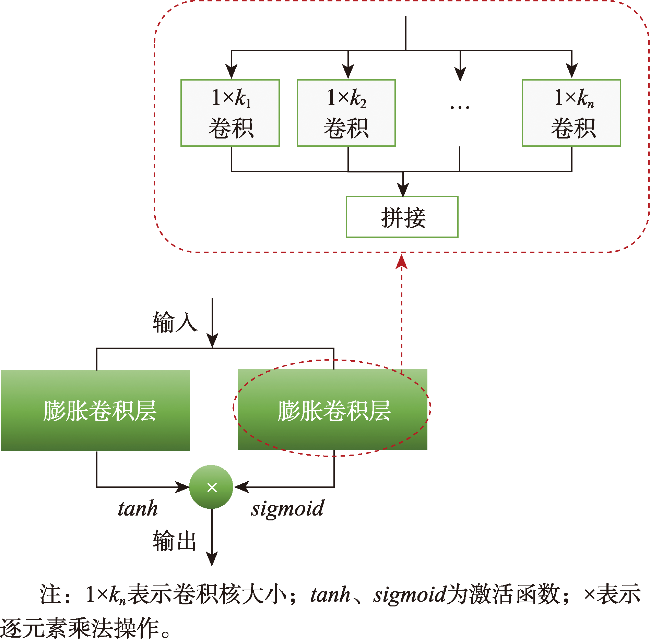
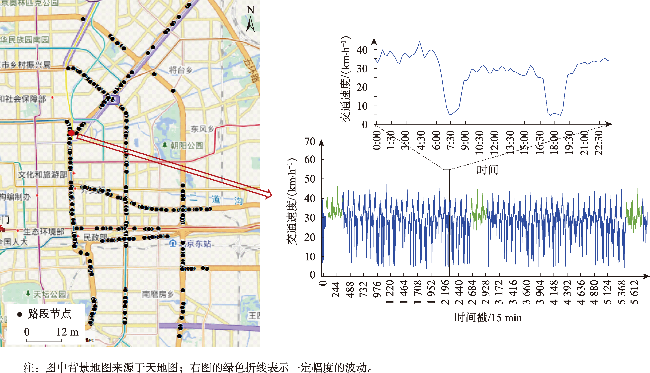
【目的】 随着城市化进程的加速和机动车数量的剧增,城市交通系统面临着巨大的压力。智能交通系统作为智慧城市的重要组成部分,被广泛应用于改善城市交通状况,交通速度预测即是其中的一个关键研究领域。实时且准确的交通速度预测对于缓解交通压力、优化交通运输和建设智能城市交通至关重要。然而城市交通网络节点间存在复杂的耦合关系和动态随机的时变特征,现有的预测方法往往难以准确捕捉其潜在的动态时空相关性。【方法】 本文将城市交通速度预测视为多变量时间序列预测问题,提出了一种基于多元时间序列动态图神经网络(MTDGNN)的交通速度预测模型。该模型基于实时交通信息,通过图学习层自适应地生成交通动态图,结合预定义的道路网络静态图,从多方面捕捉空间依赖性。同时,图卷积模块和时间卷积模块交替使用,构建多层次的空间邻域与时间感受野,充分提取交通数据的空间特征和时间特征。【结果】 本文在北京市东部城区2017年4月1日—5月31日397条路段的真实交通数据集上对 MTDGNN 模型进行了实验测试,并将预测结果与9个基准模型和7个消融实验模型进行对比。与9种基准模型相比, MTDGNN模型的平均MAE降低了至少2.24%,平均RMSE降低了至少3.98%。【结论】 MTDGNN模型在MAE、RMSE和MAPE评估指标上均取得了最优的预测精度,表明该模型在复杂交通场景中的优越性与鲁棒性。

练培格 , 李英冰 , 刘波 , 冯晓珂 . 基于多元时间序列动态图神经网络的交通速度预测[J]. 地球信息科学学报, 2025 , 27(3) : 636 -652 . DOI: 10.12082/dqxxkx.2025.240641
[Objectives] With accelerating urbanization and a surge in vehicle numbers, urban traffic systems face immense pressure. Intelligent transportation systems, a vital component of smart cities, are widely employed to improve urban traffic conditions, with traffic speed prediction being a key research focus. However, the complex coupling relationships and dynamically varying characteristics of urban traffic network nodes pose challenges for existing traffic speed prediction methods in accurately capturing dynamic spatio-temporal correlations. Spatio-temporal graph neural networks have proven to be among the most effective models for traffic speed prediction tasks. However, most methods heavily rely on prior knowledge, limiting the flexibility of spatial feature extraction and hindering the dynamic representation of road network topology. Recent approaches, such as adaptive adjacency matrix construction, address the limitations of static graphs. However, they often overlook the synergy between dynamic features and static topology, making it difficult to fully capture the complex fluctuations in traffic flow, which in turn limits prediction accuracy and adaptability. [Methods] To address these challenges, this study formulates urban traffic speed prediction as a multivariate time-series forecasting problem and proposes a traffic speed prediction model based on a Multivariate Time-series Dynamic Graph Neural Network (MTDGNN). Leveraging real-time traffic information and predefined static graph structures, the model adaptively generates dynamic traffic graphs to capture spatial dependencies through a graph learning layer and integrates them with static road network graphs to capture spatial dependencies from multiple perspectives. Meanwhile, the alternating use of graph convolution and temporal convolution modules constructs a multi-level spatial neighborhood and temporal receptive field, fully exploring the spatial and temporal features of traffic data. [Results] The MTDGNN model was tested on real traffic data from 397 road sections in eastern Beijing, collected between April 1, 2017, and May 31, 2017. Its prediction results were compared against nine benchmark models and seven ablation models. Compared to benchmark models, MTDGNN reduced the average MAE by at least 2.24% and the average RMSE by at least 3.98%. [Conclusions] Experimental results demonstrate that the MTDGNN model achieves superior prediction accuracy in MAE, RMSE, and MAPE evaluation metrics, highlighting its robustness and effectiveness in complex traffic scenarios.
表2 基线模型及其方法描述Tab. 2 Baseline models and corresponding method descriptions |
| 基线模型 | 模型方法描述 |
|---|---|
| HA | 历史平均值法,使用历史交通速度的平均值作为预测值 |
| SVR[30] | 支持向量回归法,使用线性支持向量机进行回归任务 |
| LSTM[31] | 长短期记忆网络,属于RNN,能有效捕获时序数据中的长短时非线性依赖 |
| DCRNN[32] | 基于GNN和RNN,将GRU与双向扩散卷积相结合 |
| STGCN[15] | 基于GNN和CNN,结合了图卷积和门控因果卷积,使用完全卷积结构来提取交通数据中的时空信息 |
| Conv-GCN[18] | 基于GNN和CNN,将多图卷积和三维卷积结合 |
| STAWnet[22] | 基于CNN和注意力机制,使用膨胀卷积和空间自注意力网络,来捕捉时间关联和动态空间关联 |
| ASTGCN[20] | 基于GNN和CNN,构建了一个时空注意力模块和时空卷积模块 |
| Graph WaveNet[33] | 基于GNN和CNN,使用扩散图卷积和和膨胀卷积,并提出了一种自适应邻接矩阵 |
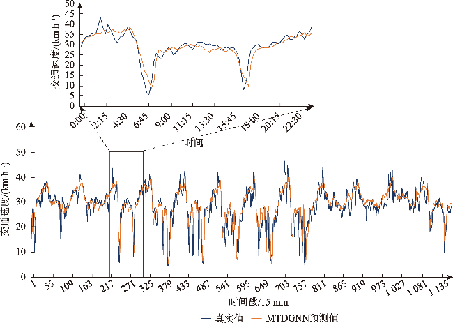
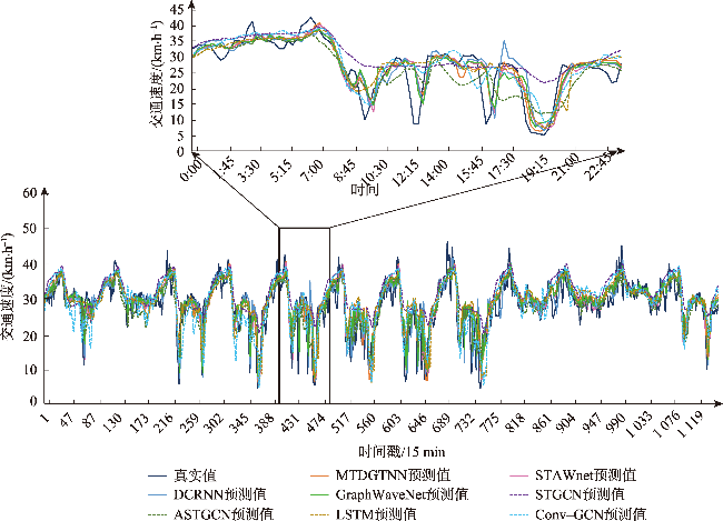
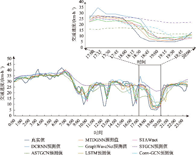
图11 路段a预测值与真实值对比Fig. 11 Comparison of predicted value and true value of road section 'a' |
表3 不同模型不同时间步长预测性能比较Tab. 3 Comparison of prediction performance of different models at different time steps |
| 方法 | 30 min | 60 min | 90 min | 120 min | |||||||||||
|---|---|---|---|---|---|---|---|---|---|---|---|---|---|---|---|
| MAE | RMSE | MAPE/% | MAE | RMSE | MAPE/% | MAE | RMSE | MAPE/% | MAE | RMSE | MAPE/% | ||||
| HA | 4.52 | 7.48 | 15.06 | 5.36 | 8.81 | 18.13 | 6.05 | 9.83 | 20.66 | 6.66 | 10.67 | 22.83 | |||
| SVR | 3.20 | 5.14 | 11.84 | 3.92 | 6.42 | 14.17 | 4.50 | 7.43 | 16.21 | 5.06 | 8.35 | 18.26 | |||
| LSTM | 3.35 | 5.78 | 12.18 | 3.37 | 5.84 | 12.30 | 3.41 | 5.89 | 12.62 | 3.46 | 6.01 | 12.91 | |||
| DCRNN | 2.56 | 4.14 | 8.36 | 3.09 | 5.25 | 10.76 | 3.25 | 5.58 | 11.47 | 3.41 | 5.85 | 12.11 | |||
| STGCN | 3.64 | 6.12 | 14.14 | 3.65 | 6.16 | 14.15 | 3.68 | 6.24 | 14.39 | 3.73 | 6.30 | 14.50 | |||
| Conv-GCN | 3.72 | 5.69 | 14.71 | 4.00 | 6.12 | 15.78 | 4.26 | 6.53 | 17.10 | 4.53 | 6.90 | 18.44 | |||
| STAWnet | 2.41 | 3.92 | 7.79 | 2.90 | 4.93 | 10.02 | 3.03 | 5.20 | 10.70 | 3.14 | 5.40 | 11.19 | |||
| ASTGCN | 3.00 | 4.65 | 10.11 | 3.60 | 5.75 | 12.75 | 3.96 | 6.37 | 14.22 | 4.33 | 6.90 | 15.63 | |||
| Graph WaveNet | 2.45 | 3.95 | 7.97 | 2.96 | 4.99 | 10.29 | 3.11 | 5.25 | 10.99 | 3.23 | 5.45 | 11.52 | |||
| MTDGNN(本文方法) | 2.39 | 3.89 | 7.92 | 2.83 | 4.85 | 9.78 | 2.96 | 5.11 | 10.28 | 3.10 | 5.34 | 10.74 | |||
注:加粗数值为对应预测步长同一指标中的最小值。 |
表4 各模块模型检验结果对比Tab. 4 Comparison of model test results of each module |
| 模型 | 平均MAE | 平均RMSE | 平均MAPE/% |
|---|---|---|---|
| w/o cross | 2.766 4 | 4.714 1 | 9.69 |
| w/o dilated | 2.788 2 | 4.808 1 | 9.61 |
| w/o mixhop | 2.687 0 | 4.652 3 | 9.35 |
| w/o gc | 2.680 2 | 4.657 8 | 9.25 |
| MTDGNN(本文方法) | 2.669 1 | 4.627 8 | 9.13 |
注:加粗数值为各模型同一指标中的最小值。 |
表5 不同图结构比较Tab. 5 Comparison of prediction results of different graph structures |
| 图结构 | 计算公式 | 公式编号 | MAE | RMSE | MAPE/% |
|---|---|---|---|---|---|
| 预定义图 | - | 2.680 2 | 4.657 8 | 9.25 | |
| 简单自适应图 | (7) | 2.673 1 | 4.653 1 | 9.22 | |
| 自注意力动态图 | (8) | 2.674 5 | 4.663 8 | 9.26 | |
| 本文提出的动态自适应图 | (9) | 2.669 1 | 4.627 8 | 9.13 |
注:表中MAE、RMSE、MAPE均为平均值;加粗数值表示各方法在同一指标中的最小值。 |
利益冲突:Conflicts of Interest 所有作者声明不存在利益冲突。
All authors disclose no relevant conflicts of interest.
| [1] |
|
| [2] |
|
| [3] |
刘静, 关伟. 交通流预测方法综述[J]. 公路交通科技, 2004, 21(3):82-85.
[
|
| [4] |
|
| [5] |
|
| [6] |
|
| [7] |
|
| [8] |
|
| [9] |
|
| [10] |
|
| [11] |
|
| [12] |
翟志鹏, 曹阳, 沈琴琴, 等. 基于多时空图融合与动态注意力的交通流预测[J/OL]. 计算机工程,1-9[2024-08-12].
[
|
| [13] |
|
| [14] |
|
| [15] |
|
| [16] |
|
| [17] |
|
| [18] |
|
| [19] |
|
| [20] |
|
| [21] |
|
| [22] |
|
| [23] |
|
| [24] |
|
| [25] |
尹宝才, 王竟成, 张勇, 等. 基于谱域超图卷积网络的交通流预测模型[J]. 北京工业大学学报, 2024, 50(2):152-164.
[
|
| [26] |
马帅, 刘建伟, 左信. 图神经网络综述[J]. 计算机研究与发展, 2022, 59(1):47-80.
[
|
| [27] |
|
| [28] |
|
| [29] |
|
| [30] |
|
| [31] |
|
| [32] |
|
| [33] |
|
| [34] |
央视网. 暑假期间北京早高峰时间延后拥堵时间延后到7至10时[EB/OL]. (2017-7-16)[2024-12-25].
[
|
| [35] |
端木一博, 柴彦威. 北京市就业者日常活动的时间利用研究——基于2007年与2017年调研数据的对比[J]. 人文地理, 2021, 36(2):136-145.
[
|
/
| 〈 |
|
〉 |
