
Journal of Geo-information Science >
Research on Chlorophyll-a Retrieval Simulation in Waters Based on the Normalized Peak Area
Received date: 2013-10-29
Request revised date: 2014-01-21
Online published: 2014-11-01
Copyright
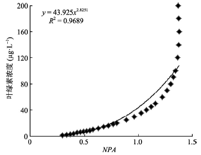
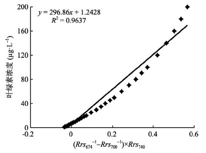
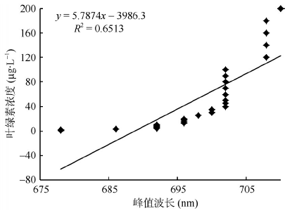
The chlorophyll-a concentration of waters is one of the main retrieval parameters in the field of water color remote sensing. Based on the coefficients of absorption and backscattering of waters, Colored Dissolved Organic Matter(CDOM), tripton and chlorophyll-a, which are achieved using the Hydrolight software package, the remote sensing reflectance is simulated according to the forward radiation transfer models without the consideration of fluorescence peak. And then, the spectral curves of variable chlorophyll-a concentration are achieved. The spectral characteristics of chlorophyll-a are analyzed according to these remote sensing reflectance curves. Next, the retrieval models of chlorophyll-a are built based on analyzing the spectral characteristics within selected bands or certain band combinations. In this paper, the Normalized Peak Area (NPA) model and three-band model are analyzed and applied to retrieve the chlorophyll-a concentration. As a comparison, other retrieval models are also considered. According to the analysis and results, we find that the chlorophyll-a concentration could be better retrieved by the NPA model, the three-band model, and a few other models, except for the model of reflectance peak position. The least competent retrieval model for chlorophyll-a is the model of reflectance peak position with the R2 of 0.6513. Among all the retrieval models, the NPA model is the best model to retrieve cholorophyll-a concentration with the R2 of 0.9689 and the RMS error of 25.25µg·L-1. The second one is the three-band model with the R2 of 0.9637 and the RMS error of 10.66µg·L-1. The small retrieval error of the three-band model is due to the consideration of the backscattering impacts of tripton, CDOM and waters. The NPA model, in addition, has not only take into consideration of the backscattering impacts, but also the fluorescence efficiency and a variety of environmental factors when applied to retrieve chlorophyll-a concentration. In the end, we could conclude that the NPA could be utilized to retrieve chlorophyll-a concentration for simulated data. This conclusion should be further verified by using it with in situ experiments data.
MA Wandong , WANG Qiao , WU Chuanqing , YIN Shoujing , XING Qianguo , ZHU Li , WU Di . Research on Chlorophyll-a Retrieval Simulation in Waters Based on the Normalized Peak Area[J]. Journal of Geo-information Science, 2014 , 16(6) : 965 -970 . DOI: 10.3724/SP.J.1047.2014.00965
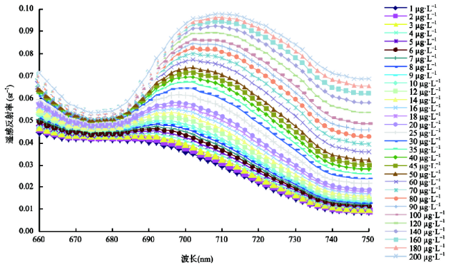
Fig.1 Reflection curves of chlorophyll-a with different concentrations in red band region图1 不同叶绿素浓度的水体在红波段的反射率变化曲线 |
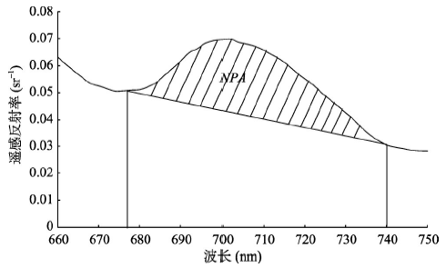
Fig.2 Illustration of the NPA in red band region图2 叶绿素红波段反射峰面积示意图 |
Fig.3 Relationship between chlorophyll-a concentration and the NPA图3 叶绿素浓度与NPA的相关关系 |
Fig.4 Relationship between chlorophyll-a concentration and the three-band model图4 叶绿素浓度和三波段模型[(Rrs674-1-Rrs700-1)×Rrs740]的相关关系 |
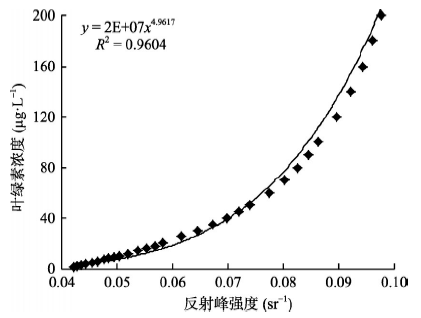
Fig.5 Relationship between chlorophyll-a concentration and the reflectance peak intensity in red band region图5 叶绿素浓度随反射峰强度的变化规律 |
Fig.6 Relationship between chlorophyll-a concentration and the wavelength of reflectance peak图6 叶绿素浓度随反射峰波长的变化规律 |
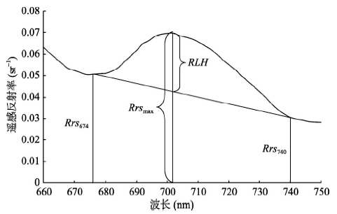
Fig.7 The illustration of the RLH图7 红光线高度示意图 |
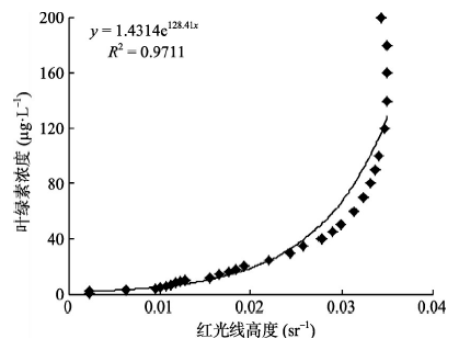
Fig.8 Relationship between chlorophyll-a concentration and RLH图8 叶绿素浓度和红光线高度的相关关系 |
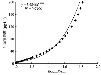
Fig.9 Relationship between chlorophyll-a concentration and Rrsmax/Rrs674图9 叶绿素浓度同Rrsmax/Rrs674的相关关系 |
Tab.1 Comparison between different chlorophyll-a retrieval models表1 水体叶绿素不同反演模型比较 |
| 反演模型 | 决定系数(R2) | 反演误差RMS(µg·L-1) |
|---|---|---|
| 反射峰面积模型 | 0.9689 | 25.25 |
| 三波段模型 | 0.9637 | 10.66 |
| 反射峰强度模型 | 0.9604 | 3.69 |
| 反射峰波长模型 | 0.6513 | 33.04 |
| 红光线高度模型 | 0.9711 | 20.62 |
| 比值模型 | 0.9356 | 10.67 |
The authors have declared that no competing interests exist.
| [1] |
|
| [2] |
|
| [3] |
|
| [4] |
|
| [5] |
|
| [6] |
|
| [7] |
|
| [8] |
|
| [9] |
|
| [10] |
|
| [11] |
|
| [12] |
|
| [13] |
|
| [14] |
|
| [15] |
|
| [16] |
|
| [17] |
|
| [18] |
|
| [19] |
|
| [20] |
|
| [21] |
|
| [22] |
|
| [23] |
|
| [24] |
|
| [25] |
|
| [26] |
|
| [27] |
|
| [28] |
|
/
| 〈 |
|
〉 |