
Journal of Geo-information Science >
Comparative Analysis of Methods of Wind Field Simulation Based on Spatial Interpolation
Received date: 2013-10-30
Request revised date: 2013-12-11
Online published: 2015-01-05
Copyright
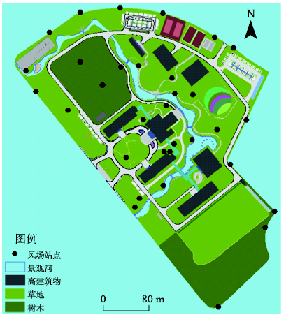
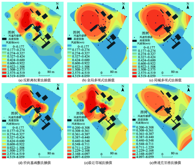
The computational fluid dynamics (CFD) method is one of the major ways of wind fields patial pattern simulation at present. This method is more often applied to wind field simulations and analyses on small scales because of the limitations of the hardware and software. Meanwhile, the precision and accuracy of this method depends on the precision of 3D building model sand the accuracy of iterated computation models, and there are significant differences existing between the simulation results and the real wind field situation. With the development of Internet of Things (IoT) technology, we can provide precise parameters to real-time simulation of regional wind fields pace distribution, by using a large number of real-time field sensor nodes. Spatial interpolation can be used to simulate the spatial distribution of all the regional environment factors. In order to determine the optimal method for real-time wind fields imulation, this research took the monthly average wind speed data of November, 2011, which are collected from 32 wind speed sensors in Institute of Urban Environment, CAS, as the example. Then, we make a comprehensive analysis of Inverse Distance Weight method, Global Polynomial method, Local Polynomial method, Radial Basis Function method, Nearest Neighbor method and Ordinary Kriging method, and compare the results of the six different methods by Cross-Validation. The result shows that the Inverse Distance Weight method is better than the other methods in the simulation error range, the simulation accuracy and the ability to reflect extreme value, which provides a reference for wind field simulation on small scales.
Key words: wind field; Internet of Things; spatial interpolation
DONG Zhinan , ZHENG Shuanning , ZHAO Huibing , DONG Rencai . Comparative Analysis of Methods of Wind Field Simulation Based on Spatial Interpolation[J]. Journal of Geo-information Science, 2015 , 17(1) : 37 -44 . DOI: 10.3724/SP.J.1047.2015.00037
Fig. 1 Spatial distribution map of wind speed monitoring stations in Institute of Urban Environment, CAS图1 中国科学院城市环境研究所风环境监测站点分布图 |
Tab. 1 Types of spatial interpolation methods表1 空间插值方法分类 |
| 确定性插值 | 地统计插值 | |
|---|---|---|
| 全局性插值 | 局部性插值 | |
| 全局多项式插值 | 反距离权重插值 | 普通克里格插值 |
| 最近邻域法插值 | 简单克里格插值 | |
| 径向基函数法插值 | 泛克里格插值 | |
| 局域多项式插值 | 概率克里格插值 | |
| 析取克里格插值 | ||
| 协同克里格插值 | ||
Fig. 2 Filled contour map of the interpolation results of monthly wind speed field (November, 2011)图2 2011年11月风速场空间插值结果 |
Tab. 2 The results of Cross-Validation error of the six interpolation methods (m/s)表2 6种插值方法的整体插值误差指标(m/s) |
| 插值方法 | MAE | MRE | RMSE |
|---|---|---|---|
| IDW | 1.454 | 2.168 | 2.272 |
| GP | 1.590 | 2.799 | 2.217 |
| LP | 1.652 | 2.947 | 2.318 |
| RBF | 1.891 | 3.795 | 2.639 |
| NN | 1.492 | 2.191 | 2.367 |
| OK | 1.684 | 2.488 | 2.674 |
Tab. 3 Observed value, correlation coefficient and the six interpolation methods (m/s, no units for correlation coefficient)表3 6种插值方法的结果与观测值的比较 |
| 数据项 | Max(m/s) | Min(m/s) | Mean(m/s) | Range(m/s) | Sd(m/s) | 相关系数 |
|---|---|---|---|---|---|---|
| 观测值 | 8.059 | 0.200 | 0.986 | 7.859 | 1.969 | 1 |
| IDW | 7.496 | 0.188 | 0.953 | 7.308 | 1.873 | 0.802 |
| GP | 3.416 | 0.051 | 1.095 | 3.366 | 1.660 | 0.792 |
| LP | 4.066 | 0.134 | 1.419 | 3.933 | 1.525 | 0.564 |
| RBF | 6.065 | 0.179 | 0.822 | 5.886 | 1.773 | 0.828 |
| NN | 7.171 | 0.192 | 0.933 | 6.949 | 1.727 | 0.804 |
| OK | 6.417 | 0.013 | 1.395 | 6.404 | 1.836 | 0.136 |
The authors have declared that no competing interests exist.
| [1] |
|
| [2] |
|
| [3] |
|
| [4] |
|
| [5] |
|
| [6] |
|
| [7] |
|
| [8] |
|
| [9] |
|
| [10] |
|
| [11] |
|
| [12] |
|
| [13] |
|
| [14] |
|
| [15] |
|
| [16] |
|
| [17] |
|
| [18] |
|
| [19] |
ESRI.Inc. Geostatistical Analyst快速浏览[EB/OL].
|
| [20] |
|
| [21] |
|
| [22] |
|
| [23] |
|
/
| 〈 |
|
〉 |