
Journal of Geo-information Science >
Impact Analysis of Land Use/Cover on Air Pollution
Received date: 2014-09-11
Request revised date: 2014-10-28
Online published: 2015-03-10
Copyright
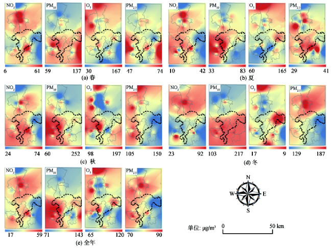
Land use/cover changes generally have complex effects on air pollution situations. Taking Chang-Zhu-Tan urban agglomeration as an example, this study investigated how do the air pollution concentrations vary with the land use/cover changes. In this process, the land use/cover was firstly retrieved from Landsat 8 images and was consequently used to calculate and map the landscape metrics. Meanwhile, concentration surfaces of PM2.5, PM10, NO2, and O3 in January, May, August and October were generated separately with the observed data from 23 stationary sites. After that, Pearson correlation coefficient was utilized to measure the relationships between concentration surfaces and land use/cover, as well as its landscape metrics. Results reveal that the highest average NO2 concentration occurred in the built-up and road areas, while the green spaces generally had lower concentrations. This situation was almost repeated by PM2.5 concentration all through the year except in spring, but was completely opposite to that of O3. However, impacts of land use/cover on PM10 concentration are relatively undeterminable due to the locally intensive industrial activities and building constructions. Analysis of landscape metrics further demonstrates that the increased index values of Perimeter-Area Fractal Dimension (PAFRAC) and Shannon Diversity (SHDI) were basically accompanied with higher PM10 and PM2.5 concentrations, respectively. Interspersion and Juxtaposition Index (IJI) were positively correlated with the concentrations of PM10, NO2, and PM2.5, however it was found negatively correlated with O3 concentration. In addition, findings from the “Ecological Green Heart” demonstration district suggest that the optimization of land use/cover pattern contributed only slightly to the decline of air pollution concentrations in this area. Therefore, it can be concluded that the air pollution concentrations in Chang-Zhu-Tan urban agglomeration were certainly influenced by its land use/cover pattern, and rational land use development activities would be helpful for reducing the air pollution concentrations in this area.
XU Shan , ZOU Bin , PU Qiang , GUO Yu . Impact Analysis of Land Use/Cover on Air Pollution[J]. Journal of Geo-information Science, 2015 , 17(3) : 290 -299 . DOI: 10.3724/SP.J.1047.2015.00290
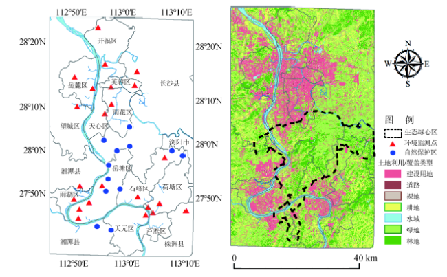
Fig. 1 The land use/land cover map of Chang-Zhu-Tan urban agglomeration图1 长株潭城市群土地利用/覆盖图 |
Tab. 1 The area proportion of different land use/land cover types in Chang-Zhu-Tan urban agglomeration and its “Ecological Green Heart” district表1 长株潭城市群及其生态绿心区各类土地利用/覆盖类型占比 |
| 总面积 (km2) | 各类土地利用/覆盖类型面积占比(%) | |||||||
|---|---|---|---|---|---|---|---|---|
| 建设用地 | 道路 | 裸地 | 耕地 | 水域 | 绿地 | 林地 | ||
| 长株潭城市群全区 | 3425.18 | 21.55 | 1.63 | 1.04 | 12.69 | 3.43 | 46.16 | 17.43 |
| 生态绿心区 | 522.87 | 11.60 | 1.06 | 0.63 | 9.31 | 4.32 | 55.08 | 18.00 |
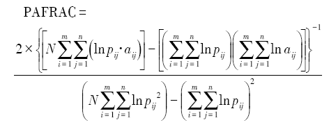
Fig. 2 The spatial distribution patterns of landscape metrics in Chang-Zhu-Tan urban agglomeration图2 长株潭城市群景观指数空间分布格局 |
Fig. 3 The spatial distribution patterns of NO2、PM10、O3、PM2.5 concentrations in different seasons and the annual mean value in Chang-Zhu-Tan urban agglomeration图3 长株潭城市群NO2、PM10、O3、PM2.5季节和年均浓度空间分布格局 |
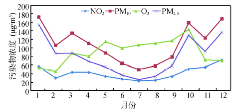
Fig. 4 The monthly concentration change of air pollution in Chang-Zhu-Tan urban agglomeration in 2013图4 长株潭城市群2013年空气污染浓度月均变化趋势 |
Fig. 5 Seasonal and mean annual concentrations of NO2、PM10、O3、PM2.5 under various land use/land cover types in Chang-Zhu-Tan urban agglomeration图5 长株潭城市群各类土地利用/覆盖类型NO2、PM10、O3、PM2.5季节和年均浓度统计均值(单位:ug/m3) |
Tab. 2 The correlation coefficients of air pollution concentrations and PLAND in Chang-Zhu-Tan urban agglomeration表2 长株潭城市群各类型土地占比(PLAND)与空气污染浓度的相关系数 |
| NO2 | PM10 | ||||||||||
|---|---|---|---|---|---|---|---|---|---|---|---|
| 年均 | 春季 | 夏季 | 秋季 | 冬季 | 年均 | 春季 | 夏季 | 秋季 | 冬季 | ||
| 建设用地 | 0.34* | 0.31* | 0.23* | 0.22* | 0.27* | -0.08* | -0.06* | -0.02 | -0.07* | 0.03 | |
| 道路 | 0.21* | 0.13* | 0.19* | 0.29* | 0.07 | 0.09 | 0.05 | 0.17* | 0.11 | 0.06 | |
| 裸地 | -0.07 | -0.06 | -0.10 | -0.10 | 0.04 | -0.06 | -0.08 | 0.01 | -0.07 | 0.02 | |
| 耕地 | -0.16* | -0.15* | -0.14* | -0.14* | -0.11* | -0.07* | -0.01 | -0.16* | -0.08* | -0.08* | |
| 水域 | -0.03 | 0.03 | 0.04 | -0.07 | -0.06 | 0.05 | -0.04 | 0.03 | 0.06 | 0.06 | |
| 绿地 | -0.01 | -0.04 | -0.05* | 0.04 | 0.01 | 0.04 | 0.01 | 0.12* | 0.02 | 0.06* | |
| 林地 | -0.34* | -0.33* | -0.27* | -0.26* | -0.26* | 0.12* | 0.30* | -0.13* | -0.05 | 0.06 | |
| O3 | PM2.5 | ||||||||||
| 年均 | 春季 | 夏季 | 秋季 | 冬季 | 年均 | 春季 | 夏季 | 秋季 | 冬季 | ||
| 建设用地 | -0.16* | -0.02 | -0.14* | -0.21* | -0.26* | 0.32* | 0 | 0.09* | 0.14* | 0.34* | |
| 道路 | -0.04 | -0.01 | -0.14* | 0.07 | -0.16* | 0.13* | 0 | 0.16* | -0.01 | 0.08 | |
| 裸地 | 0.11 | 0.14 | 0.13 | 0.04 | 0.07 | -0.07 | -0.12 | -0.19* | 0.13 | -0.02 | |
| 耕地 | -0.01 | -0.05 | 0.11* | 0.07* | -0.08* | -0.06 | 0.07* | -0.12* | -0.02 | -0.07* | |
| 水域 | 0.02 | 0.10* | 0 | 0.05 | -0.06 | 0.03 | -0.11* | -0.05 | 0.28* | -0.05 | |
| 绿地 | 0.08* | 0.02 | 0.03 | -0.07* | 0.29* | -0.16* | -0.06* | 0.03 | -0.22* | -0.07* | |
| 林地 | -0.20* | -0.31* | -0.02 | 0.16* | -0.21* | -0.19* | 0.30* | -0.14* | -0.24* | -0.26* | |
*表示在0.01水平上显著相关 |
Tab. 3 The correlation coefficients of air pollution concentrations and landscape metrics in Chang-Zhu-Tan urban agglomeration表3 长株潭城市群土地利用景观指数与空气污染浓度的相关系数 |
| NO2 | PM10 | ||||||||||
|---|---|---|---|---|---|---|---|---|---|---|---|
| 年均 | 春季 | 夏季 | 秋季 | 冬季 | 年均 | 春季 | 夏季 | 秋季 | 冬季 | ||
| CONTAG | -0.02 | -0.02 | -0.05 | -0.05 | 0.09* | -0.02 | 0.04 | 0.00 | -0.04 | 0.05 | |
| IJI | 0.10* | 0.11* | 0.12* | 0.07 | 0.01 | -0.05 | -0.05 | -0.04 | -0.05 | -0.05 | |
| PAFRAC | -0.01 | -0.11* | 0.12* | 0.32* | -0.36* | 0.30* | 0.33* | 0.16* | 0.35* | -0.07 | |
| AI | 0.00 | 0.03 | -0.02 | -0.11* | 0.11* | -0.04 | -0.06 | 0.02 | -0.08 | 0.08 | |
| SHDI | 0.05 | 0.01 | 0.06 | 0.08 | -0.06 | 0.03 | -0.04 | 0.04 | 0.06 | 0.00 | |
| O3 | PM2.5 | ||||||||||
| 年均 | 春季 | 夏季 | 秋季 | 冬季 | 年均 | 春季 | 夏季 | 秋季 | 冬季 | ||
| CONTAG | 0.11* | 0.10* | 0.06 | -0.03 | 0.22* | -0.06 | -0.09* | 0.10* | -0.08 | -0.07 | |
| IJI | -0.12* | -0.05 | -0.10* | 0.00 | -0.24* | 0.14* | 0.06 | 0.01 | 0.11* | 0.12* | |
| PAFRAC | -0.02 | -0.10* | -0.22* | 0.28* | -0.11* | 0.04 | 0.19* | 0.17* | 0.01 | -0.11* | |
| AI | 0.06 | 0.07 | 0.09* | -0.09* | 0.13* | -0.04 | -0.08 | -0.01 | -0.03 | 0.01 | |
| SHDI | -0.05 | -0.02 | -0.06 | 0.06 | -0.18* | 0.13* | 0.06 | -0.08 | 0.17* | 0.11* | |
*表示在0.01水平上显著相关 |
The authors have declared that no competing interests exist.
| [1] |
|
| [2] |
|
| [3] |
|
| [4] |
|
| [5] |
|
| [6] |
|
| [7] |
|
| [8] |
|
| [9] |
|
| [10] |
|
| [11] |
|
| [12] |
|
| [13] |
|
| [14] |
|
| [15] |
|
| [16] |
|
| [17] |
|
| [18] |
USGS Global Visualization Viewer. 遥感影像[DB/OL]. 2013-12-12].
|
| [19] |
|
| [20] |
|
| [21] |
|
| [22] |
|
| [23] |
|
| [24] |
|
| [25] |
|
| [26] |
|
| [27] |
|
/
| 〈 |
|
〉 |

