Orginal Article

Scale Transformation Algorithm for Remote Sensing Imagery Based on Greatest Common Divisor

  • GAO Yonggang* ,
  • XU Hanqiu
Expand
  • 1. College of Environment and Resources, Fuzhou University, Fuzhou 350108, China
  • 2. Institute of Remote Sensing Information Engineering, Fuzhou University, Fuzhou 350108, China
*Corresponding author: GAO Yonggang, E-mail:

Received date: 2015-05-11

  Request revised date: 2015-08-03

  Online published: 2015-12-20

Copyright

《地球信息科学学报》编辑部 所有

Abstract

The abundant remote sensing data with various spatial, radiational and spectral resolutions from multi-platforms provide rich information sources for the study of land surface information changes at different scales. Scale variation and sensitivity have a great impact on the application of remote sensing imagery in different scientific fields. We proposed a transformation algorithm to unify the scales for comparing data at different scales. The method is a scale transformation algorithm based on the greatest common divisor (STAGCD). Firstly, the greatest common divisor (GCD) between two different spatial scales is calculated. Secondly, according to the GCD, a GCD image will be produced by resampling the original remote sensing image. Finally, the new scale image will be obtained according to certain intervals for row and column to choose data from the GCD image. Several scale transformation algorithms have been employed in the test of the scale unification for an IKONOS image, including STAGCD and some other algorithms from professional software packages, such as ER Mapper, ERDAS, Matlab and so on. The effectiveness of these algorithms has been evaluated based on the information keeping degree compared with the original remote sensing image. A total of six indicators have been used for quantitative evaluation of the scale transformed images. The histogram and probability density function of Gauss based on kernel bandwidth optimization have been used for visual interpretation of the scale transformed images. The results show that the STAGCD image has adequate ability for keeping the information of original image. When scaling-down, STAGCD only increases the image size, but cannot improve the image’s spatial resolution. When scaling-up, STAGCD not only reduces the image size, but also decreases the image resolution. The STAGCD method is simple and can transform remote sensing imagery at different scales. The method provides an effective solution for the scale transformation between images without an integer multiple relationship.

Cite this article

GAO Yonggang* , XU Hanqiu . Scale Transformation Algorithm for Remote Sensing Imagery Based on Greatest Common Divisor[J]. Journal of Geo-information Science, 2015 , 17(12) : 1520 -1528 . DOI: 10.3724/SP.J.1047.2015.01520

1 引言

尺度是指研究对象或现象在空间上的量度,即空间尺度[1]。Cao和Lam在Lam和Quattrochi对空间域尺度划分的基础上,进一步将空间域尺度细分为地图尺度(Cartographic or Map Scale)、地理尺度(Geographic or Observational Scale)、测量尺度(Measurement Scale)和运行尺度(Operational Scale)[2]。对于遥感影像而言,尺度的概念可理解为遥感影像的空间分辨率、光谱分辨率、辐射分辨率和时间分辨率。遥感影像的空间分辨率与地理学中的地图尺度相关。地表景观间的差异和变化主要用其空间细节和整体性表现。因此,遥感影像的应用尺度主要为空间分辨率对地物景观描述的研究。
遥感应用的尺度研究涉及尺度效应、尺度转换和尺度选择3个方面的内容,其中,尺度转换是指利用某种算法生成不同空间分辨率的遥感影像或进行遥感影像空间分辨率的统一,即空间分辨率的缩放或空间分辨率的统一。空间分辨率的缩放是指将单一空间分辨率的遥感影像按照一定的转换算法生成不同空间分辨率遥感影像的过程。空间分辨率的统一是指将同源或异源遥感卫星上,不同空间分辨率的遥感影像统一到相同空间分辨率的过程。空间分辨率缩放包括向上尺度转换(Upscaling)和向下尺度转换(Downscaling)。向上尺度转换也称为尺度扩展,是指将高空间分辨率遥感影像转换为低空间分辨率的过程,其主要方法有统计方法和地学机理方法[4]。统计方法有局部平均法、中值法、中心法及重采样法(最近邻法、双线性内插和立方卷积内插)、统计分形等相关算法[5-16]。地学机理方法是通过建立多个变量的模型来预测低分辨率上某一地学变量的值,因此,这种模型需除去被转换变量以外的其他辅助信息[1],且该模型会因转换信息而异。向下尺度转换也称为尺度收缩,是指将低空间分辨率遥感影像转换为高空间分辨率遥感影像的过程,最常用的方法为遥感影像融合[17]
遥感影像的尺度研究主要是针对同幅遥感影像,且其空间分辨率缩放过程中获得的遥感影像均为原始遥感影像空间分辨率的整倍数关系,很少涉及非整倍数关系。对于空间分辨率缩放算法研究较多,而对于空间尺度统一问题的研究则较少。因此,本文提出了最大公约数的空间尺度转换方法。

2 影像空间尺度转换原理与方法

2.1 空间尺度统一

遥感影像处理中经常会遇到不同空间分辨率之间进行变化检测和数据比较等问题,而其首先须进行空间尺度的统一。如果2幅遥感影像间的空间分辨率是整倍数关系,则其空间尺度转换相对简单,直接采用最邻近像元法等插值算法进行重采样即可;但当2幅遥感影像间的空间分辨率为非整倍数关系时(如空间分辨率为4 m的IKONOS遥感影像和空间分辨率为10 m的SPOT遥感影像),此时通常不能直接进行转换。
为了解决空间分辨率为非整倍数关系的遥感影像间空间尺度的统一问题,本文提出以下解决方法:首先,将遥感影像重采样(尺度下推,即下采样)生成不同空间分辨率的最大公约数遥感影像;然后,利用相关算法重采样(尺度上推,即上采样)生成所需空间分辨率遥感影像。重采样到指定空间分辨率遥感影像后的行、列数,其计算公式如式(1)、(2)所示。
Ro w r = int Ro w o × R o R r (1)
Co l r = int Co l o × R o R r (2)
式中,Rowr为重采样后遥感影像的行数;Colr为重采样后遥感影像的列数;Rowo为原遥感影像总行数,Colo为原遥感影像的总列数;Ro为原遥感影像的空间分辨率;Rr为重采样后遥感影像的空间分辨率;int( )为取整函数。
2.1.1 最大公约数
最大公约数(Greatest Common Divisor,GCD)为几个整数共有因子中最大的一个,其计算公式如式(5)所示。
GCD = gcd R 1 × 10 n , R 2 × 10 n 10 n (3)
式中,GCD为最大公约数;gcd( )为最大公约数计算方法,常用的gcd( )计算方法有短除法、辗转相除法(欧几里得算法)、质因数分解法和列举法等;R1R2为2幅遥感影像各自的空间分辨率;n为空间分辨率的小数位数。当R1R2均为整数时,n=0;当R1R2中只有一个为小数时,n为其小数位数;当R1R2均为小数时,n为小数位数的最大值。
2.1.2 重采样
遥感影像进行重采样的常用算法有最邻近像元法、双线性插值法和三次卷积插值法等,它们各有优缺点。最邻近像元法具有遥感影像光谱信息保持好的特点,因此,本研究采用最邻近像元法进行下采样。根据计算出的最大公约数,采用最邻近像元法将遥感影像下采样生成空间分辨率为最大公约数的遥感影像,然后采用行列剔除法、均值法、中值法或中点法等方法,对最大公约数的遥感影像进行上采样,生成指定分辨率的遥感影像。
(1)最大公约数遥感影像
计算最大公约数旨在获得多尺度遥感影像间的过渡遥感影像,以实现数据重采样后遥感影像尺寸大小和空间尺度的统一问题。
下采样生成最大公约数遥感影像时,其采样间隔计算公式如式(4)所示 。
R = R O GCD (4)
式中, R 为下采样间隔;GCD为最大公约数;Ro为原遥感影像空间分辨率;采用最邻近像元法获得的各像元的像元值,其重采样公式为式(5)-(7)。
img_GCD ( R i + d : R i + R , C j + d : C j + R ) = img_O ( i , j ) (5)
R i = i - d × R (6)
C j = j - d × R (7)
式中,img_GCD为下采样后获得的最大公约数遥感影像;img_O为原始遥感影像;i,j为原始遥感影像的行、列号; R i C j 为最大公约数遥感影像中与ij对应的行、列起始位置。d为常数,当遥感影像矩阵从(1,1)开始时取1;从(0,0)开始时,取0。
(2)指定空间分辨率遥感影像
上采样生成指定空间分辨率遥感影像时,采样间隔和遥感影像起始位置的计算公式分别如式(8)-(10)所示。
R = R r GCD (8)
Ro w = int R 2 + d (9)
Co l = int R 2 + d (10)
式中, R 为上采样间隔;GCD为最大公约数; Ro w 为行的起始位置; Co l 为列的起始位置。
行列剔除法为根据一定的采样间隔进行数据的选取,即根据式(9)和式(10)确定的遥感影像起始位置,每隔 R 个行列对遥感影像进行重采样。均值法、中值法和中点法与行列剔除法的区别为:分别利用采样间隔确定的 R × R 窗口数据的均值、中值或窗口中心点值代替行列所在处的像元值。
采用行列剔除法获得的指定空间分辨率遥感影像的像元值(式(11)-(13))。
img_New ( m , n ) = img_GCD ( R m , C n ) (11)
其中, R m = Ro w + m - d × R (12)
C n = Co l + n - d × R (13)
式中,img_New为上采样后获得的指定空间分辨率遥感影像;m,m为指定空间分辨率遥感影像的行、列号; R m C n 为最大公约数遥感影像与mn对应的行、列位置。

2.2 尺度转换评价方法

空间尺度转换精度的评价是建立在转换前后信息损失最小的基础上,通常采用地统计学方法、景观指数法等进行评价[18]。因此,本文选取统计分析中的均值(Mean)、标准差(Standard Deviation,STD)、系统偏差(System Deviation,SD)、均方根误差(Root Mean Square Error,RMSE)、相对整体维数综合误差(Erreur Relative Globale Adimensionnelle de Synthèse,ERGAS)、相关系数(Correlation Coefficient,CC)6个评价指标对尺度转换精度进行定量评价,并引入Gauss概率密度分布函数,分别对原始影像和尺度转换后获得影像的直方图进行分布函数逼近,以获取各波段的分布函数模拟图。同时,采用最优核带宽法(Kernel Bandwidth Optimization,KBO)[19]对Gauss概率密度分布函数进行最佳逼近,并绘制原始影像和尺度转换后获得的影像的直方图和Gauss概率密度分布函数的模拟图(简称Gauss分布函数图)进行目视对比分析,以提高利用直方图对光谱保真度进行目视判读的准确性。
(1)均值:为影像像元值的灰度平均值,反映了影像的平均亮度(式(14))。
Mean = r = 1 M c = 1 N I ( r , c ) M × N (14)
式中,I为遥感影像;rc为影像的行列号;MN为影像总的行列数。
(2)标准差:反映了影像相对于均值的离散程度(式(15))。
STD = r = 1 M c = 1 N I r , c - Mean 2 M × N (15)
(3)系统偏差:指原始影像与尺度变换后影像之间差值绝对值的平均值(式(16))。该值反映了尺度变换后影像与原始影像的整体差异程度,其值越小表示差异越小,理想值为0。
SD = 1 MN r = 1 M c = 1 N I ( r , c ) - I ( r , c ) (16)
式中,I为原始遥感影像; I 为尺度转换后获得的影像。
(4)均方根误差:反映了不同影像对应波段间的差异程度(式(17))。
RMSE = r = 1 M c = 1 N I r , c - I r , c 2 M × N (17)
(5)相对整体维数综合误差:ERGAS是在均方根误差RMSE的基础上,将各波段的RMSE与均值做比值,综合考察影像间的光谱差异,理想值为0。其公式如式(18)所示。
ERGA S i = 100 RMS E i 2 I ̅ i (18)
式中, I ̅ 为尺度转换后获得影像的均值; RMS E i 为影像间的均方根误差;i表示波段。
(6)相关系数:反映了不同影像对应波段间的吻合度,该值越大则表明对应波段间的吻合度越好。当相关系数为1时,则表明影像对应波段的吻合度达到最大。相关系数的计算公式如式(19)所示。
C C i = r = 1 M c = 1 N I i r , c - I ̅ i I i r , c - I ̅ i r = 1 M c = 1 N I i r , c - I ̅ i 2 × r = 1 M c = 1 N I ' i r , c - I ̅ i 2 (19)
式中, I ̅ 为原始遥感影像的均值。

3 遥感影像空间尺度转换算法实验与分析

由于经尺度变换后获得的遥感影像尺寸大小与原始影像不一致,并且在尺度变换过程中涉及像元值重采样的问题,因此,无法直接比较尺度变换前后影像的光谱信息,所以本文采用间接比较的方法(图1)。首先对原始影像进行下采样获得指定分辨率的遥感影像;然后将该影像进行尺度转换获得与原始影像相同尺度的影像;最后对这2幅影像进行评价比较。ER Mapper、ERDAS、ENVI、PCI等商业遥感软件,以及Matlab中的imresize命令,均可进行空间尺度的转换,经实验表明它们的尺度转换结果均相同,但商业遥感软件进行尺度转换时,其影像的文件信息中必须含有其空间尺度信息,否则无法按照要求的尺度进行转换。本文将利用上述专业软件进行空间尺度转换的方法简称为商业(软件)算法。
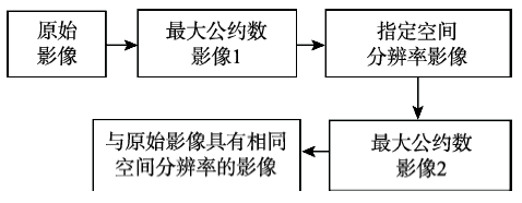
Fig. 1 Flowchart of indirect comparison method

图1 间接比较法流程图

为了验证本文所提算法的可行性及其对原始影像信息的高保真性,以IKONOS(4 m)的多光谱影像(像元大小为450×300)为数据源,选取商业(软件)算法和本文算法的空间尺度转换结果进行实验分析研究(图2)。为了使尺度转换过程中光谱信息损失最小,商业(软件)算法中重采样方法选用最邻近像元法,本文算法采用行列剔除法。在交叉变换中,如果采用商业(软件)算法将空间分辨率为4 m的原始遥感影像经尺度转换(下采样)变为0.6 m、1.5 m、2.1 m和3 m 4种尺度的影像,然后采用本文算法将上述尺度影像转换(上采样)为4 m尺度影像则该转换过程称为“商业(软件)算法→本文算法”;反之,称为“本文算法→商业(软件)算法”。如果交叉变换过程始终采用同一种算法,转换过程直接以算法名称命名。
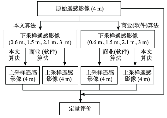
Fig. 2 Flowchart of scale transformation experiment

图2 尺度转换实验流程图

根据IKONOS各波段间的相关性,选择了4、3、1的波段组合方式对尺度转换后的各影像进行显示(Nir、Red、Blue)(图3)。限于篇幅,尺度转换后的各影像和直方图,仅以2.1 m尺度与4 m尺度的相互转换为例,同时直方图对比图中仅给出了差异较大的Nir波段的直方图和Gauss概率密度分布函数的模拟图(图4)。图3(b)-(e)为采用相应算法由2.1 m尺度影像经尺度逆变换获得的与原始影像相同尺度的影像。表1-4为原始影像与各尺度转换后影像定量评价表。
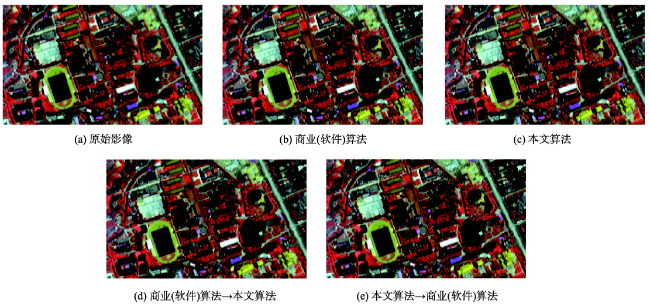
Fig. 3 Original and scale transformation imageries of IKONOS (Scale: 2.1 m)

图3 IKONOS原始影像与尺度转换后影像(尺度:2.1 m)

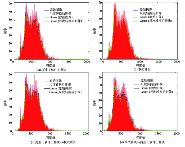
Fig. 4 Comparison diagram of histogram of original and scale transformation imageries (Scale: 2.1 m)

图4 IKONOS原始影像与各尺度转换后影像直方图对比图(尺度:2.1 m)

Tab. 1 Quantitative evaluation of the scale transformation algorithms (Scale: 2.1 m)

表1 IKONOS原始影像与尺度转换后影像定量评价表(尺度: 2.1 m)

方法 波段 评价指标
Mean STD SD RMSE ERGAS CC
原始影像 1 457.501 88.939 - - - -
2 499.650 134.548 - - - -
3 378.310 153.395 - - - -
4 504.025 174.153 - - - -
商业(软件)算法 1 457.658 89.127 25.827 52.062 11.376 0.859
2 499.956 134.772 40.693 77.405 15.482 0.835
3 378.582 153.520 46.246 85.474 22.577 0.845
4 505.493 174.515 68.193 116.083 22.964 0.779
本文算法 1 457.501 88.939 0.000 0.000 0.000 1.000
2 499.650 134.548 0.000 0.000 0.000 1.000
3 378.310 153.395 0.000 0.000 0.000 1.000
4 504.025 174.153 0.000 0.000 0.000 1.000
商业(软件)算法→本文算法 1 457.324 88.954 4.622 19.211 4.201 0.977
2 499.254 134.478 7.528 30.255 6.060 0.974
3 377.748 153.117 8.740 35.321 9.350 0.973
4 503.760 174.071 12.328 49.902 9.906 0.959
本文算法→商业(软件)算法 1 457.532 89.015 17.269 40.397 8.829 0.896
2 499.827 134.672 27.521 61.326 12.272 0.895
3 378.413 153.496 31.270 67.517 17.837 0.903
4 505.196 174.238 47.259 91.853 18.218 0.860
Tab. 2 Quantitative evaluation of the scale transformation algorithms (Scale: 0.6 m)

表2 IKONOS原始影像与尺度转换后影像定量评价表(尺度: 0.6 m)

方法 波段 评价指标
Mean STD SD RMSE ERGAS CC
原始影像 1 457.501 88.939 - - - -
2 499.650 134.548 - - - -
3 378.310 153.395 - - - -
4 504.025 174.153 - - - -
商业(软件)算法 1 457.627 89.206 18.418 42.521 9.291 0.893
2 499.810 134.880 29.469 64.073 12.820 0.886
3 378.526 153.714 33.565 71.888 18.991 0.890
4 504.407 174.265 49.750 100.117 19.848 0.834
本文算法 1 457.501 88.939 0.000 0.000 0.000 1.000
2 499.650 134.548 0.000 0.000 0.000 1.000
3 378.310 153.395 0.000 0.000 0.000 1.000
4 504.025 174.153 0.000 0.000 0.000 1.000
商业(软件)算法→本文算法 1 457.683 89.222 15.082 35.732 7.807 0.925
2 499.734 134.973 23.810 53.983 10.803 0.920
3 378.419 153.820 27.105 59.563 15.740 0.916
4 504.108 174.187 39.576 79.526 15.776 0.896
本文算法→
商业(软件)算法
1 457.600 89.072 17.133 40.822 8.921 0.899
2 499.773 134.750 27.604 61.405 12.286 0.898
3 378.509 153.654 31.560 69.278 18.303 0.897
4 504.139 174.248 46.784 97.203 19.281 0.844
Tab. 3 Quantitative evaluation of the scale transformation algorithms (Scale: 1.5 m)

表3 IKONOS原始影像与尺度转换后影像定量评价表(尺度: 1.5 m)

方法 波段 评价指标
Mean STD SD RMSE ERGAS CC
原始影像 1 457.501 88.939 - - - -
2 499.650 134.548 - - - -
3 378.310 153.395 - - - -
4 504.025 174.153 - - - -
商业(软件)算法 1 457.537 88.939 19.808 43.908 9.597 0.893
2 499.698 134.478 31.727 66.310 13.270 0.878
3 378.434 153.370 36.363 74.707 19.741 0.882
4 504.384 174.331 53.269 103.042 20.429 0.826
本文算法 1 457.501 88.939 0.000 0.000 0.000 1.000
2 499.650 134.548 0.000 0.000 0.000 1.000
3 378.310 153.395 0.000 0.000 0.000 1.000
4 504.025 174.153 0.000 0.000 0.000 1.000
商业(软件)算法→本文算法 1 457.370 88.746 17.231 40.888 8.940 0.898
2 499.360 134.352 27.665 61.670 12.350 0.895
3 378.085 153.354 31.828 69.785 18.458 0.890
4 503.460 174.258 46.045 95.918 19.052 0.849
本文算法→商业(软件)算法 1 457.456 88.861 18.961 42.756 9.348 0.901
2 499.597 134.493 30.226 64.901 12.996 0.882
3 378.419 153.359 34.431 71.901 19.015 0.889
4 504.299 174.313 52.045 97.358 19.338 0.843
Tab. 4 Quantitative evaluation of the scale transformation algorithms (Scale: 3 m)

表4 IKONOS原始影像与尺度转换后影像定量评价表(尺度: 3 m)

方法 波段 评价指标
Mean STD SD RMSE ERGAS CC
原始影像 1 457.501 88.939 - - - -
2 499.650 134.548 - - - -
3 378.310 153.395 - - - -
4 504.025 174.153 - - - -
商业(软件)算法 1 457.370 88.746 17.311 40.973 8.955 0.899
2 499.360 134.352 27.686 61.452 12.297 0.896
3 378.085 153.354 31.668 69.343 18.320 0.891
4 503.460 174.258 46.766 97.201 19.279 0.845
本文算法 1 457.501 88.939 0.000 0.000 0.000 1.000
2 499.650 134.548 0.000 0.000 0.000 1.000
3 378.310 153.395 0.000 0.000 0.000 1.000
4 504.025 174.153 0.000 0.000 0.000 1.000
商业(软件)算法→本文算法 1 457.468 89.035 11.533 34.388 7.517 0.935
2 499.554 134.604 18.368 51.286 10.266 0.929
3 378.162 153.450 21.182 58.116 15.368 0.910
4 504.145 174.560 29.918 77.752 15.423 0.901
本文算法→商业(软件)算法 1 457.392 88.787 17.091 40.755 8.910 0.900
2 499.400 134.412 27.427 61.422 12.299 0.896
3 378.131 153.421 31.565 69.502 18.381 0.897
4 503.449 174.265 45.571 95.478 18.965 0.850
通过图3分析可知,IKONOS原始影像与尺度转换后,各影像在光谱信息和空间分辨率方面无任何差别。图4(b)中,本文算法所获得的尺度转换影像与原始影像的直方图和Gauss概率密度分布图完全一致,表明2幅影像完全相同;而其他方法获得的尺度转换影像与原始影像的直方图和Gauss概率密度分布函数图均存在差异,且单一的商业(软件)算法差异最大,表明该方法在尺度转换过程中信息丢失较多。
由定量分析可知(表1-4),尺度转换后各影像与原始影像相比,本文算法获得影像的Mean和STD与原始影像完整一致,SD、RMSE和ERGAS均为0,CC为1,表明2幅影像完全相同,该计算结果与图4的分析结论相吻合;商业(软件)算法的Mean和STD的计算结果与原始影像相差最大,SD、RMSE、ERGAS和CC均与理想值相差较大,表明该结果与原始影像的相似性相差较大。在尺度转换过程中利用到本文算法时,其评价结果较单一商业(软件)算法结果的信息保持质量有所提高。此外,经另外实验表明当需转换的空间尺度为整数倍关系时,商业(软件)算法和本文算法均能对原始影像信息具有很好的保持特性,且二者的尺度转换结果完全相同;商业(软件)算法(除Matlab软件)在空间尺度转换过程中均要求原始影像的属性信息中包含对空间尺度的描述,否则其不能准确地生成指定空间尺度的影像。
本文提出最大公约数的遥感影像空间尺度转换方法,在影像尺度转换过程中很好地实现了遥感影像信息的保持,克服了专业软件对影像须包含空间分辨率信息的限制,实现了影像向任意尺度的转换。

4 结论

(1)最大公约数的空间尺度转换方法,很好地解决了遥感影像间空间分辨率为非整倍数关系时的空间尺度缩放和空间尺度统一问题,为多源、多尺度遥感影像间的数据比对研究提供了数据转换的基础。
(2)通过尺度转换后影像的定量评价和定性分析可知,本文所提的空间尺度转换算法,在非整倍数关系的尺度转换过程中,能很好地保持影像原始信息;在整倍数关系的尺度转换过程中,本文算法与商业(软件)算法具有相同的转换结果。
(3)最大公约数的空间尺度转换方法与其他常用尺度转换算法一样,在尺度下推(即下采样)过程中仅增加影像的尺寸大小,不会提高影像的空间分辨率;但在尺度上推(即上采样)过程中,在减少影像尺寸的同时,会降低影像的空间分辨率。
(4)本文算法原理简单且易于编程实现,可快速地解决遥感影像间空间分辨率的变换和统一问题。

The authors have declared that no competing interests exist.

[1]
张景雄. 空间信息的尺度、不确定性与融合[M].武汉:武汉大学出版社,2008.

[2]
Lam N, Quattrochi D A.On the issues of scale, reolution, and fractal analysis in the mapping sciences[J]. Professional Geographer, 1992,44(1):88-98.

[3]
邬建国. 景观生态学——格局、过程、尺度与等级[M].北京:高等教育出版社,2007.

[4]
柏延臣,王劲峰.遥感信息不确定性研究:分类与尺度效应模型[M].北京:地质出版社,2003.

[5]
Justice C O, Markham B L, Townshend J R G, et al. Imagery degradation of satellite data[J]. International Journal of Remote Sensing, 1989,10(9):1539-1561.

[6]
Hay G J, Niemann K O, Goodenough D G.Imagery thresholds, image-objects, and upscaling: A multi-scale evaluation[J]. Remote Sensing of Environment, 1997,62(1):1-19.

[7]
Bian L, Butler R.Comparing effects of aggregation methods on statistical and imagery properties of simulated imagery data[J]. Photogrammetric Engineering and Remote Sensing, 1999,65(1):73-84.

[8]
Kim G, Barros A P.Downscaling of remotely sensed soil moisture with a modified fractal interpolation method using contraction mapping and ancillary data[J]. Remote Sensing of Environment, 2002,83(3):400-413.Previous work showed that remotely sensed soil moisture fields exhibit multiscaling and multifractal behavior varying with the scales of observations and hydrometeorological forcing (Remote Sens. Environ. 81 (2002) 1). Specifically, it was determined that this multiscaling behavior is consistent with the scaling of soil hydraulic properties and vegetation cover, while the multifractal behavior is associated with the temporal evolution of soil moisture fields. Here, we apply these findings by directly incorporating information on the spatial structure of soil texture and vegetation water content to the spatial interpolation of remotely sensed soil moisture data.A downscaling model is presented which consists of a modified fractal interpolation method based on contraction mapping. This methodology is different from other fractal interpolation schemes because it generates unique fractal surfaces. It is different from other contraction mapping models because it includes spatially and temporally varying scaling functions as opposed to single-valued scaling factors. The scaling functions are linear combinations of the spatial distributions of ancillary data. The model is demonstrated by downscaling soil moisture fields from 10 to 1 km resolution using remote-sensing data from the Southern Great Plains 1997 (SGP'97) field experiment.

DOI

[9]
Goward S N, Davis P E, Fleming D, et al.empirical comparison of Landsat 7 and IKONOS multispectral measurements for selected Earth Observation System (EOS) validation sites[J]. Remote Sensing of Environment, 2003,88:80-99.The Space Imaging IKONOS observatory may provide an important benefit in terrestrial scientific research. The five-band, 1 m panchromatic and 4 m multispectral measurements have the potential to provide a source of measurements to evaluate subpixel land cover variability in measurements from observatories such as Landsat 7 Enhanced Thematic Mapper Plus (ETM+) and Terra MODIS sensor. The IKONOS observations are at a spatial scale equivalent to field measurements typically carried out in ecological and land cover research. As such, the IKONOS observations may serve as a source of ''virtual'' ground measurements, for the lower spatial resolution, global observatories. In this study we examine how well IKONOS sensor observations replicate Landsat 7 ETM+ visible/near infrared observations for selected Earth Observation System (EOS) validation sites in the United States. The sites examined--Beltsville, MD, Konza Prairie, KS, and Sevilleta, NM--sample the east - west moisture gradient across the United States. Observations for each site were acquired, as nearly time-coincident as possible, from ETM+ and the IKONOS sensor, several times over the growing season. This was done to insure that we compared these two sensors over the widest range of observing conditions possible. We also examined IKONOS imagery from Phoenix, AZ, where Space Imaging had and had not applied a modulation transfer function compensation (MTFC) process. The MTFC is their standard product. We found that this product, at the original 4 m spatial resolution, appears to have minor radiometric artifacts as a result of the process. When the IKONOS observations were aggregated to 30 m, this problem was essentially absent, allowing us to proceed with the remainder of our study. We processed the IKONOS sensor and ETM+ measurements to produce close approximates of each other. Our processing steps included ortho-rectification, calibration to planetary reflectance, pixel alignment and pixel aggregation. We initially found radiometric differences between the two sensors that increased with increasing wavelength. Space Imaging updated their calibration information, based on analyses from NASA Stennis Space Center staff, which removed much of this discrepancy. We now find that the IKONOS red and near infrared measurements differ between the two sensors, with IKONOS generally producing higher reflectance in the red band and lower reflectance in the near infrared band than the Landsat 7 ETM+ sensor. This results in the IKONOS sensor producing lower spectral vegetation index measurements, for the same target, than ETM+, a measurement variation that has been observed between other sensors. We also encountered far more cirrus cloud (and shadow) contamination in these paired observations that we had expected. After careful initial selection, we lost over half of our image pairs from the analysis because of cirrus cloud contamination. We do not know whether this is simply because of the paired, comparative design of this study or whether it relates to the increased spatial and radiometric resolution of the IKONOS sensor. The results of this study not only provide a baseline assessment of IKONOS versus Landsat 7 ETM+ visible and near infrared measurements but also suggest some of the issues that need more attention when comparing other sensor systems as well as developing the design of future land observatories.

DOI

[10]
Wang G, Gertner G, Anderson A B.Up-scaling methods based on variability-weighting and simulation for inferring imagery information across scales[J]. International Journal of Remote Sensing, 2004,25(22):4961-4979.

[11]
彭晓娟,邓孺孺,刘小平.遥感尺度转换研究进展[J].地理与地理信息科学,2004,20(5):6-14.造成遥感问题复杂化的重要原因 之一就是不同遥感测量方式获取的数据及地面测量数据在尺度上的不一致。在应用不同尺度的遥感数据时 ,尺度转换显得格外重要。该文阐述了遥感尺度转换所解决的问题 ,并针对国内外研究现状 ,分别论述基于像元和基于对象的遥感尺度转换的研究进展 ,对各种尺度转换方法的转换效果进行分析。最后对遥感尺度转换研究的发展趋势与前景进行展望

DOI

[12]
布仁仓,李秀珍,胡远满,等.尺度变换的正确率分析[J].生态学报,2004,24(4):659-665.采用优势规则和随机规则为基础的尺度分析方法 ,对分类的 TM数据 (景观类型图 ,包含 8类型 )进行了尺度变换分析。随着尺度的增加 ,优势规则分析方法使景观中优势景观类型的面积增加 ,相反 ,面积较小的非优势景观类型的面积减少。随机规则使各景观类型的面积基本上保持不变。随着尺度的增加 ,随机 K appa指数、位置 Kappa指数和标准 Kappa指数减少。在优势规则分析法中数量 Kappa指数减少 ,但在随机规则为基础的处理中它保持 10 0 %。优势规则处理中的正确率大于随机规则处理的。由景观类型的面积百分比引起的数量正确率在优势规则处理中增加 ,但在随机规则处理中保持 9.6 4 %不变 ;相反数量错误在优势规则处理中明显增加 ,但在随机规则处理中少量增加。偶然正确率保持 12 .5 0 %不变。位置正确率减少 ,相反位置错误明显增加。层和亚层水平上的位置正确率和错误的变化不明显 ,而网格水平上的位置正确率和错误大幅度减少。网格水平上的位置正确率和错误率决定了整个位置正确率和错误率 ,同时位置正确率和错误率基本上决定了整个正确率和错误率。标准Kappa指数大于等于 70 %作为选择依据 ,认为 2 10m是优势规则处理法的尺度阈值,150m是随机规划处理法的尺度阈值,欲提高尺度阈值,必须改变研究范围或分类系统。

[13]
韩鹏,龚健雅,李志林,等.遥感影像空间尺度上推方法的评价[J].遥感学报,2008,12(6):965-971.首先分析了几种常用的影像质量评价指标在遥感数据空间尺度上推方 法评价中的不足,同时提出了已有的关于空间尺度上推方法在评价思路上的不妥之处.引入了空间分辨率和SSIM(structural SIMilarity)2个遥感影像质量评价指标,给出了新的评价思路,并在此基础上对5种遥感数据空间尺度转换方法进行了评价.在本实验中,空间分辨率 和SSIM 2个遥感影像质量评价指标一致表明,Bilinear和Bicubic方法的结果影像能够更好地接近目标空间尺度下的影像特征.实验表明,依据新的评价思 路,采用空间分辨率和SSIM 2个评价指标进行空间尺度上推方法表现出较强的有效性和优越性.

DOI

[14]
Hubert S, Schwarzer S, Jaquet J M.Imagery degradation of classified satellite images[J]. The Open Remote Sensing Journal, 2012,5:64-72.

[15]
胡云锋,徐芝英,刘越,等.地理空间数据的尺度转换[J].地球科学进展, 2013,28(3):297-304.<p>尺度一般是指空间范围的大小,地理空间数据的尺度转换是尺度研究的重要问题之一。针对地理信息系统(GIS)技术支持下的地理空间数据尺度转换问题,首先回顾了尺度转换的理论基础,即等级理论、分形理论、区域化随机变量理论、地理学第一定律等理论的基本内涵;然后总结了地理学不同研究领域内主要的尺度转换方法,重点分析了重采样法、变异函数法、分形分维法及小波分析法的基本原理、模型方法与典型应用案例;最后介绍了地理空间数据尺度转换效应研究的进展。基于上述总结和分析认为:构建一套无级变换的、系统的尺度转换方法,整合不同学科领域的数据与过程模型、形成数据模型同化的技术体系,这是地理空间数据尺度转换研究的重要课题。</p>

[16]
栾海军,田庆久,余涛,等.基于分形理论的NDVI连续空间尺度转换模型研究[J].光谱学与光谱分析,2013,33(7):1857-1862.尺度效应是遥感领域的一个非常重要的科学问题。定量遥感尺度转换研究可用于解决如定量遥感反演产品真实性检验等诸多颇具挑战性的问题。传统升尺度转换研究方法无法得到连续空间尺度上反演量的变化特性;且面临不同传感器间几何、光谱等特性参数校正问题的干扰,尺度转换研究精度受到影响。为此,基于分形理论利用单一传感器影像解决这些问题。基于Enhanced Thematic Mapper Plus(ETM+)数据,以NDVI(利用其地表辐亮度计算模型)为研究对象,建立了一个可参考的反演量连续空间尺度转换模型研究流程。结果表明:(1)NDVI升尺度转换中存在尺度效应,且此效应可由尺度转换分形模型定量描述;(2)此分形模型适用于NDVI产品的真实性检验中。这表明分形作为一种有效的方法,可用于定量遥感尺度转换研究中。

DOI

[17]
布和敖斯尔,马建文,王勤学,等.多传感器不同分辨率遥感数字图像的尺度转换[J].地理学报,2004,59(1):101-110.<p>针对日益增多的多传感器不同分辨率的遥感数字图像数据,提出其综合利用和尺度转换的有效方法。其中,作为尺度上推 (scaling-up) 技术,本研究选择IHS和小波分解变换两种数据融合方法,应用Landsat ETM+数据和IRS-1C数据进行了实例研究。发现: IHS方法操作简单,对两种待融合的图像的像元大小和像元数 (bit数) 的依赖不是很高,而对原始图像光谱信息的依赖很高,因此适用于不同传感器之间的数据融合上,其缺点就是不能够更多的保留原始多光谱数据的光谱信息。小波分解变换 (WD) 方法可以很好地保留多光谱传感器的所有光谱信息,但是在重采样中对两种待融合的图像的像元配准的要求很高,因此比较适合于对同一传感器的多光谱数据与全色光谱数据的融合上。作为尺度下退 (scaling-down) 技术,通过探讨将札幌野外实验站点数据镶嵌到高时间分辨率遥感图像的问题,提出像元级尺度扩展的具体操作方法和对NDVI图像进行扩展时出现混合像元的识别方法。应用AVHRR, MODIS, ETM+和ASTER的NDVI图像数据进行了像元尺度的扩展研究。得出: 对不同传感器的不同分辨率的数据之间进行像元级的尺度扩展后,能够较好地识别出不同地物的分布边界,较好的分辨混合像元,因此其结果可用于对不同地物分布特征的分类研究或土地覆盖变化中的时间序列变化的研究中。</p>

[18]
徐芝英,胡云锋,刘越,等.空间尺度转换数据精度评价的准则和方法[J].地理科学进展,2012,31(12):1574-1582.空间尺度问题是地理学、生态学和水文学等多个学科的基础科学问题之一。空间数据尺度转换是将数据从一个空间尺度转换到另一个空间尺度的过程, 它是尺度科学研究的重要内容之一。对尺度转换后的成果数据深入分析, 提炼尺度转换成果数据精度评价的原则、指标以及模型方法, 这对正确选择和应用尺度转换成果数据具有重要意义。在详细评述尺度和尺度转换研究概念、内容和主要进展的基础上, 本文主要从数据处理、地图学角度出发, 提出了空间数据尺度转换精度评价的3 项基本准则, 即保持构成信息守恒、保持面积信息守恒、保持区域空间格局和形态信息守恒。继而据此将当前常见的指标进行了梳理和归并;根据上述准则和指标, 结合GIS 方法、常规统计方法、地统计方法等, 给出了上述评价指标的计算模型及其应用方法和典型案例。最后指出, 在实际应用中需结合研究目标, 针对性选择尺度转换效应函数, 通过开展模型模拟和对比分析, 最终确定合适的尺度转换方法。

DOI

[19]
Shimazaki H, Shinomoto S.Kernel bandwidth optimization in spike rate estimation[J]. Journal of Computational Neuroscience, 2010,29:171-182.Kernel smoother and a time-histogram are classical tools for estimating an instantaneous rate of spike occurrences. We recently established a method for selecting the bin width of the time-histogram, based on the principle of minimizing the mean integrated square error (MISE) between the estimated rate and unknown underlying rate. Here we apply the same optimization principle to the kernel density estimation in selecting the width or &#8220;bandwidth&#8221; of the kernel, and further extend the algorithm to allow a variable bandwidth, in conformity with data. The variable kernel has the potential to accurately grasp non-stationary phenomena, such as abrupt changes in the firing rate, which we often encounter in neuroscience. In order to avoid possible overfitting that may take place due to excessive freedom, we introduced a stiffness constant for bandwidth variability. Our method automatically adjusts the stiffness constant, thereby adapting to the entire set of spike data. It is revealed that the classical kernel smoother may exhibit goodness-of-fit comparable to, or even better than, that of modern sophisticated rate estimation methods, provided that the bandwidth is selected properly for a given set of spike data, according to the optimization methods presented here.

DOI PMID

Outlines

/