
Journal of Geo-information Science >
Effect of Outcrop Sampling Density on the Underlying Terrain Reconstruction
Received date: 2015-03-11
Request revised date: 2015-03-29
Online published: 2016-04-19
Copyright
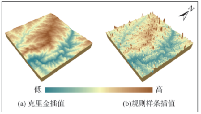
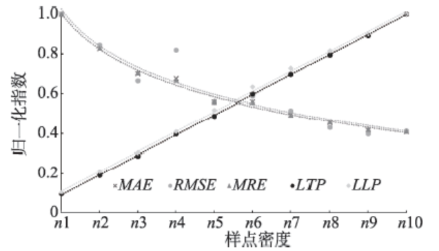
The Pre-Quaternary underlying terrain profoundly controls the evolution and formation of loess landform. Obvious relationships, i.e. the geomorphological inheritance, could be found between the underlying terrain and the modern terrain. As a consequence, the Pre-Quaternary underlying terrain in the Loess Plateau should be regarded as the key factor for the understanding of the loess landform evolution. Among numerous numerical calculation methods, spatial interpolation has been regarded as an important method to reconstruct the DEM of underlying terrain by using the sampled bedrock outcrop points selected from a geological map. However, the sampling density has a great impact on the accuracy of the reconstructed underlying terrain. In this paper, the Suide geological map area (1:200 000) was selected as the study area, and then the influence of sampling density on the accuracy of the reconstructed underlying terrain was investigated using spline method. By adopting cross-validation method to evaluate reconstructed underlying terrain, the result shows that, different interpolation methods cause uncertainties to different degrees during the reconstruction of underlying terrain, particularly the spline method. On a basis of high density outcrop points and spline function interpolation process, the morphology of underlying terrain exhibits a typical “Runge phenomenon”. This phenomenon was always resulted from a polynomial interpolation process. With an increased sampling density, the error in underlying terrain appears a slowly decrease tendency firstly, and then it keeps stable. Meanwhile, the number of the extracted features has a linear upward trend. The result also shows that the sampling density of 1.7-2.0 points per square kilometer could achieve a good balance between the accuracy and underlying terrain feature reservation. The aforementioned results adjust our previous understandings that spline function could smooth the interpolated surface to some extent. And the result also provides guidance for the selection of a reasonable spatial sampling density.
Key words: DEM; Loess underlying terrain; sampling density; spline interpolation
DUAN Jiazhen , XIONG Liyang , TANG Guoan . Effect of Outcrop Sampling Density on the Underlying Terrain Reconstruction[J]. Journal of Geo-information Science, 2016 , 18(4) : 461 -468 . DOI: 10.3724/SP.J.1047.2016.00461
Fig. 1 Interpolation results of by Kriging function and regular spline function under high sampling density图1 高密度样点条件下普通克里金函数与规则样条函数插值结果对比 |
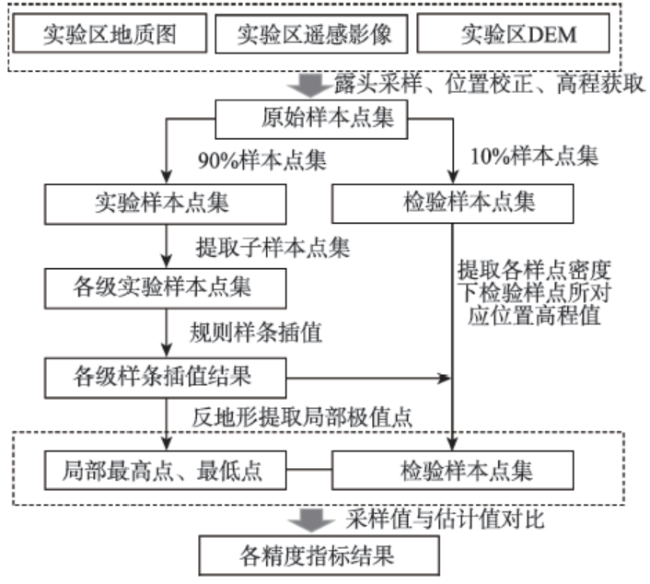
Fig. 2 Flow chart of this research图2 实验流程图 |
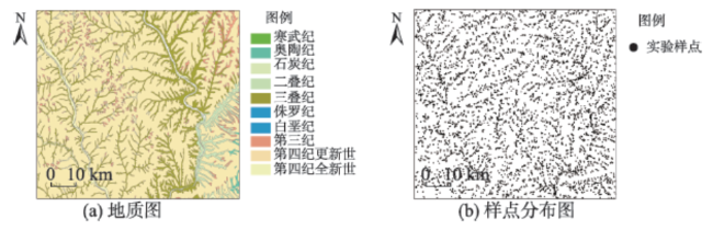
Fig. 3 Geological map of the study area and the distribution of samplings图3 实验样区地质图及样本点分布图 |
Tab. 1 Numbers of samplings and their equivalent density in each dataset表1 各样本点集样本点数及等效密度表 |
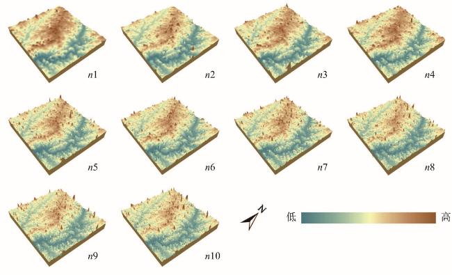
| 样本集 | n1 | n2 | n3 | n4 | n5 | n6 | n7 | n8 | n9 | n10 |
|---|---|---|---|---|---|---|---|---|---|---|
| 点数 | 2531 | 5061 | 7592 | 10 122 | 12 653 | 15 183 | 17 714 | 20 244 | 22 775 | 25 305 |
| 等效密度/(个/km2) | 0.346 | 0.693 | 1.040 | 1.386 | 1.733 | 2.080 | 2.427 | 2.773 | 3.120 | 3.466 |
Fig. 4 Reconstructed results of the underlying terrain under different sampling density图4 各样点密度古地形重建结果 |
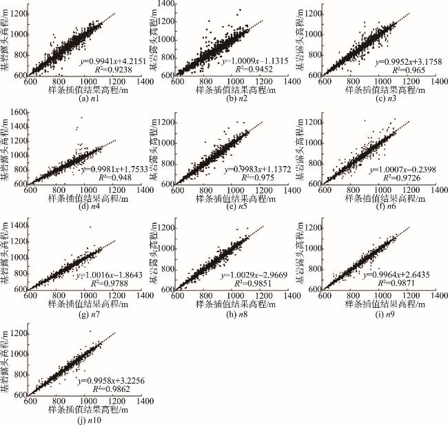
Fig. 5 XY scatter diagram for the measured value and estimated value under different sampling density图5 不同样本集下检验样点的实测值与估计值XY散点图 |
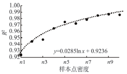
Fig. 6 Correlation coefficient for the measured value and the estimated value of the test samples图6 检验样点的实测值与估计值相关系数 |
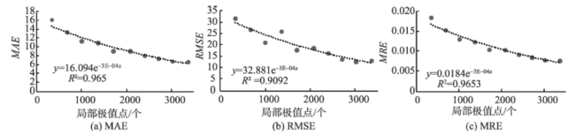
Tab. 2 Error statistics under different sampling density表2 各样点密度下插值结果精度误差统计表 |
| 样本集 | n1 | n2 | n3 | n4 | n5 | n6 | n7 | n8 | n9 | n10 |
|---|---|---|---|---|---|---|---|---|---|---|
| MAE | 16.132 | 13.325 | 11.295 | 10.912 | 9.032 | 9.032 | 8.004 | 7.343 | 6.718 | 6.587 |
| RMSE | 31.647 | 26.701 | 21.030 | 25.904 | 17.708 | 18.607 | 16.358 | 13.654 | 12.612 | 13.060 |
| MRE | 0.018 | 0.015 | 0.013 | 0.012 | 0.010 | 0.010 | 0.009 | 0.008 | 0.007 | 0.007 |
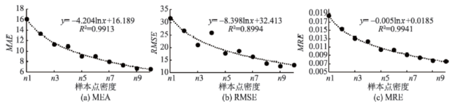
Fig. 7 Error statistic under different sampling density图7 各样点密度下精度误差 |
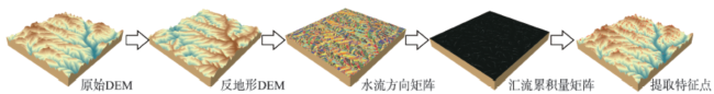
Fig. 8 Flow chart of LHP extraction method based on reverse DEM图8 反地形DEM局部最高点提取流程图 |
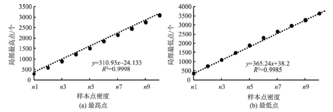
Tab. 3 Number of LHPs and LLPs number with different sampling density表3 各样点密度下局部最高点和最低点统计表 |
| 样本集 | n1 | n2 | n3 | n4 | n5 | n6 | n7 | n8 | n9 | n10 |
|---|---|---|---|---|---|---|---|---|---|---|
| LHP | 300 | 589 | 895 | 1234 | 1515 | 1853 | 2158 | 2457 | 2762 | 3097 |
| LLP | 370 | 761 | 1105 | 1493 | 1895 | 2308 | 2650 | 2968 | 3279 | 3641 |
Fig. 9 Number of LHPs and LLPs with different sampling density图9 各样点密度下局部最高点与局部最低点 |
Fig. 10 Relation between local extreme value and each precision index图10 各精度指标与局部极值点相关图 |
Fig. 11 Each precision result normalization with different sampling density图11 不同样点密度下各精度结果归一化图 |
The authors have declared that no competing interests exist.
| [1] |
[
|
| [2] |
[
|
| [3] |
[
|
| [4] |
[
|
| [5] |
[
|
| [6] |
[
|
| [7] |
[
|
| [8] |
|
| [9] |
|
| [10] |
|
| [11] |
|
| [12] |
|
| [13] |
|
| [14] |
|
| [15] |
[
|
| [16] |
[
|
| [17] |
[
|
| [18] |
|
| [19] |
[
|
| [20] |
[
|
| [21] |
[
|
| [22] |
[
|
| [23] |
[
|
| [24] |
[
|
/
| 〈 |
|
〉 |