
Journal of Geo-information Science >
Finite Element Numerical Simulation Method of Groundwater Flow and Its Application under 3D GIS
Received date: 2015-07-02
Request revised date: 2015-11-09
Online published: 2016-06-10
Copyright
The existing finite element numerical simulation method of groundwater flow has some defects in the three-dimensional visual spatial analysis and the expression of numerical calculation process and simulation results. In order to solve this issue, the key steps of the finite element analysis process including the conceptual model construction, spatial discretization, hydrogeological parameters extraction and initial condition assignment are taken into consideration respectively. Based on the finite element method and 3D GIS platform, the method and technique framework of the groundwater finite element numerical simulation under 3D GIS are proposed with the supports of GIS spatial analysis algorithms and computer graphics theory. In addition to describe the technique framework, the core algorithms’ implementation details are given and the complete process of 3D GIS groundwater flow simulation is presented. The groundwater simulation example demonstrates that the proposed method and technique framework are capable of simplifying the finite element analysis process and improving the calculation efficiency of the model. The whole technique framework can be integrated into 3D GIS platform, and furthermore the visualization of simulation process and calculation results can be achieved eventually.
MA Junting , CHEN Suozhong , ZHU Xiaoting , HE Zhichao . Finite Element Numerical Simulation Method of Groundwater Flow and Its Application under 3D GIS[J]. Journal of Geo-information Science, 2016 , 18(6) : 749 -757 . DOI: 10.3724/SP.J.1047.2016.00749
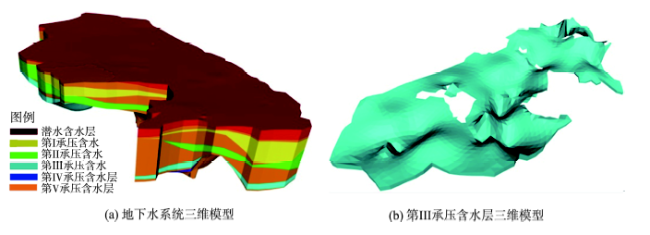
Fig. 1 3D groundwater system and the III aquifer data model of the study area图1 研究区地下水系统及第III承压含水层的三维空间数据模型 |
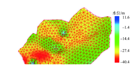
Fig. 2 Hydraulic gradient adapted finite element mesh图2 随水力梯度模自适应的自适应有限元离散格网 |
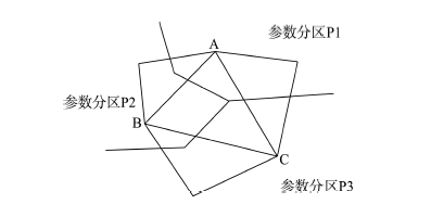
Fig. 3 Diagram of single mesh element overlapping multiple parameter districts图3 格网单元压覆多个参数分区示意图 |
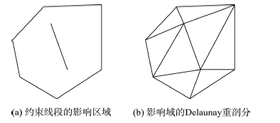
Fig. 4 Diagram of triangular mesh topological local reconstruction图4 三角网的局部重建原理示意图 |
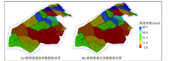
Fig. 5 Comparison of parameter extraction before and after the mesh local reconstruction图5 格网重建前后渗透系数提取结果对比图 |
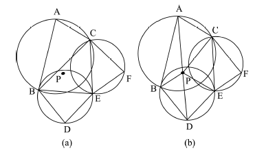
Fig. 6 Diagram of inserting a point into the triangular mesh图6 点插入算法原理示意图 |
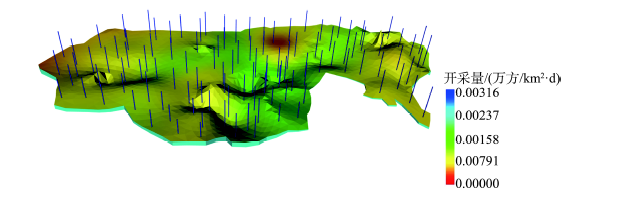
Fig. 7 Visualization of the initial water level and assignment of the exploitation values图7 初始水位和开采量赋值的可视化效果图 |
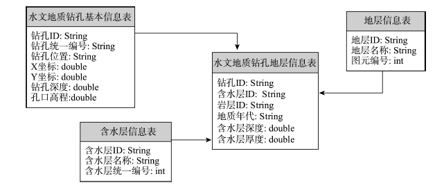
Fig. 8 Standard database structure of hydro-geological bore data图8 水文地质钻孔标准数据库结构 |
Tab. 1 Parameters of the groundwater finite element numerical model表1 地下水有限元数值模型参数数据说明表 |
| 参数名称 | 空间类型 | 属性来源 |
|---|---|---|
| 含水层地层描述信息 | 点要素 | 水文地质钻孔数据库 |
| 初始水位 | 点要素 | 动态历史水位数据库 |
| 渗透系数、导水系数、贮水系数 | 面要素 | 水文地质专题图 |
| 参数分区(河流、断层等约束线) | 线要素 | 水文地质专题图 |
| 开采量 | 点要素 | 历史开采量数据库 |
| 越流补给系数、侧向补给系数 | 面要素 | 用户输入 |
Tab. 2 Comparison table of the actual and calculated results表2 水位计算值与实测值对比表 |
| 井号 | 时段水位/m | ||||||||||||||
|---|---|---|---|---|---|---|---|---|---|---|---|---|---|---|---|
| 2014-10-15 | 2014-11-15 | 2014-12-15 | 2015-01-14 | ||||||||||||
| 实测 | 计算 | 误差 | 实测 | 计算 | 误差 | 实测 | 计算 | 误差 | 实测 | 计算 | 误差 | ||||
| 1 2 3 4 5 6 7 8 9 10 11 12 13 14 15 | -22.07 -8.13 -21.42 -4.25 -3.23 -6.01 -25.32 -24.92 -38.89 -33.56 -24.69 2.37 -19.84 -24.80 -24.06 | -22.08 -8.14 -21.41 -4.24 -3.20 -6.00 -25.34 -24.90 -38.88 -33.57 -24.70 2.35 -19.83 -24.81 -24.07 | -0.01 -0.01 0.01 0.01 -0.03 0.01 -0.02 0.02 0.01 -0.01 -0.01 -0.02 0.01 -0.01 -0.01 | -22.07 -8.13 -21.42 -4.25 -3.23 -6.01 -25.32 -24.92 -38.89 -33.56 -24.69 2.37 -19.84 -24.80 -24.06 | -22.76 -8.86 -21.29 -4.90 -3.74 -6.60 -25.94 -25.80 -38.45 -33.77 -23.84 -2.87 -19.22 -24.97 -23.64 | -0.69 -0.73 0.13 -0.65 -0.51 -0.59 -0.62 -0.88 0.44 -0.21 0.85 -0.50 0.62 -0.17 0.42 | -22.07 -8.13 -21.42 -4.25 -3.23 -6.01 -25.32 -24.92 -38.89 -33.56 -24.69 -2.37 -19.84 -24.80 -24.06 | -20.50 -7.33 -20.22 -4.98 -1.27 -4.52 -24.69 -23.59 -37.73 -34.34 -23.08 -3.10 -18.42 -24.42 -22.34 | 1.57 0.80 1.20 -0.73 1.96 1.49 1.63 1.33 1.16 -0.78 1.61 -0.73 1.42 0.38 1.72 | -21.95 -7.99 -21.92 -4.09 -2.77 -6.18 -25.36 -24.70 -36.03 -33.89 -23.38 -3.96 -19.73 -21.75 -25.36 | -20.76 -6.44 -20.05 -3.61 -1.13 -4.92 -26.08 -22.75 -35.03 -33.11 -24.90 -3.68 -19.52 -22.82 -23.62 | 1.19 1.55 1.87 0.48 1.64 1.26 -1.72 1.95 1.00 0.78 -1.52 0.28 0.21 -1.07 1.74 | |||
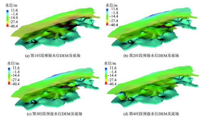
Fig. 9 Prediction result visualization of time intervals from 1 to 4图9 第1-4时段的预报结果可视化 |
The authors have declared that no competing interests exist.
| [1] |
|
| [2] |
|
| [3] |
|
| [4] |
|
| [5] |
|
| [6] |
|
| [7] |
[
|
| [8] |
[
|
| [9] |
[
|
| [10] |
[
|
| [11] |
[
|
| [12] |
[
|
| [13] |
[
|
| [14] |
|
| [15] |
[
|
| [16] |
[
|
| [17] |
[
|
| [18] |
[
|
| [19] |
[
|
| [20] |
|
| [21] |
|
| [22] |
|
| [23] |
[
|
| [24] |
[
|
/
| 〈 |
|
〉 |