Orginal Article

An Applicability Study of Covariance Localization Method in ETKF Data Assimilation

  • HAN Pei 1 ,
  • SHU Hong , 1, * ,
  • XU Jianhui 2 ,
  • WANG Jianlin 3
Expand
  • 1. State Key Laboratory of Information Engineering in Surveying, Mapping and Remote Sensing, Wuhan University, Wuhan 430079, China
  • 2. Guangdong Open Laboratory of Geospatial Information Technology and Application, Guangzhou Institute of Geography, Guangzhou 510070, China
  • 3. Soil and Water Conservation Monitoring Center of Hubei Province, Wuhan 430071, China
*Corresponding author: SHU Hong, E-mail:

Received date: 2015-07-09

  Request revised date: 2016-01-12

  Online published: 2016-09-27

Copyright

《地球信息科学学报》编辑部 所有

Abstract

To explore the applicability of the covariance localization method in the Ensemble Transform Kalman Filter (ETKF) scheme, we firstly analyze some difficulties of the covariance localization method applied to the ETKF scheme in theory. In order to solve the current problem, then we develop an approximate covariance localization method for ETKF, which is accomplished through the Schur product on ensemble perturbations, and finally we test the suitability and the effect of the approximate covariance localization method in ETKF by combining the Lorenz - 96 model. This model is often used to do performance evaluation in data assimilation. The results show that the covariance localization method cannot be directly applied to ETKF assimilation, although it can eliminate some spurious correlations in the background error covariance matrix and increase the rank of the background error covariance matrix. Because the effective object of Schur product in the covariance localization method is the background error covariance matrix, but the update equations of the ETKF only contain the ensemble perturbation matrix, excluding the background error covariance matrix. Moreover, the dimensions between the correlation coefficient matrix and the ensemble perturbation matrix are different, so an approximate covariance localization method is developed. By the experiment, it shows that the approximate covariance localization method can be applied in the ETKF, but the approximate Schur product disrupts the dynamic balances of ETKF assimilation system ,which leads to bad assimilation results. The local analysis method is widely used to solve the localization problem in data assimilation systems, so we try to apply it into the ETKF scheme. The results show that the local analysis method can be directly applied to ETKF, it can remove the spurious correlations in background error covariance matrix and obtain better assimilation results. This paper is a theoretical innovation and experimental exploration, it helps the related researchers to do further studies on the localization in the data assimilation.

Cite this article

HAN Pei , SHU Hong , XU Jianhui , WANG Jianlin . An Applicability Study of Covariance Localization Method in ETKF Data Assimilation[J]. Journal of Geo-information Science, 2016 , 18(9) : 1184 -1190 . DOI: 10.3724/SP.J.1047.2016.01184

ETKF)同化的适用性,本文在理论上分析了CL方法应用于ETKF同化存在的困难,发展了一种适用于ETKF同化的对集合扰动进行舒尔积运算的近似CL方法,并结合Lorenz-96模型对近似CL方法的适用性及其对同化结果的影响进行了分析。研究结果表明:CL方法不仅能消除背景误差协方差矩阵中的伪相关,还能增加背景误差协方差矩阵的秩,但CL方法并不能直接用于ETKF同化;近似CL方法可应用于ETKF同化中,但近似舒尔积破坏了ETKF同化系统的动态平衡,导致同化结果误差较大;与CL方法相反,局地化分析(Local Analysis,LA)方法可直接应用于ETKF同化,并能较好地消除ETKF同化的背景误差协方差矩阵的伪相关,获得较优的同化结果。
关键词:协方差局地化;集合转换卡尔曼滤波;同化;伪相关

1 引言

卡尔曼滤波(Kalman Filter,KF)是顺序数据同化算法的最早形式和理论基础,在线性系统和高斯白噪声条件下可得到无偏最优估计,其背景误差协方差矩阵具有“流依赖”[1](flow-dependent)特征。但是,大气预报模式多数是非线性系统,且状态变量维数巨大(O(107)),误差统计的计算量无法满足。因此,KF的应用受到极大限制。1994年Evensen提出了集合卡尔曼滤波(Ensemble Kalman Filter,EnKF),它用有限集合的误差统计近似表示背景误差统计。研究表明,EnKF不仅能较好地体现背景误差协方差的“流依赖”特征,而且能有效地减少误差统计计算量,降低预报误差。在EnKF的实际应用中,为了防止背景误差协方差减小过快、出现滤波发散,通常对集合样本加入观测扰动,观测样本误差的引入导致EnKF成为一种次优滤波。因此,相关学者发展了不加入观测扰动的确定性滤波,如确定性卡尔曼滤波(Deterministic Ensemble Kalman Filter,DEnKF)[2]、集合均方根滤波(Ensemble Square Root Filter,EnSRF)[3]、集合转换卡尔曼滤波(Ensemble Transform Kalman Filter,ETKF)[4]等。ETKF最初是由Bishop等[4]针对适应性观测问题提出,后来被Wang等[5]用于集合预报初值扰动的生成,Wei等[6]应用到实际同化业务中。与其它集合同化方案不同,ETKF可用集合变换和标准化观测算子快速地估计出与观测网有关的背景误差协方差矩阵。
在集合数据同化中,有限的集合数目和相同的集合成员设置,会使2个本应无关或者实际相关性很低的状态变量之间产生虚假或过高的相关。因为每个集合成员相当于对当前大气真实状态的一种采样,大气自由度过高,完全采样不切实际;另外,模式存在系统的误差,相同的集合成员设置会有相似的系统误差,这使集合成员的预报在某些方面有一致性,从而产生伪相关[7]。为了解决伪相关的问题,使观测只对附近的状态变量产生影响,局地化在数据同化中被采用。目前,局地化分为2种方式:(1)基于背景误差协方差的局地化,如协方差局地化方法(Covariance Localization,CL),通过在背景误差协方差矩阵上乘以一个局地化算子,改变背景误差协方差矩阵[3,8];(2)观测误差协方差局地化,如局地分析方法[9](Local Analysis,LA),通过在观测误差协方差矩阵上乘以一个随距离增加的函数,增大观测方差,间接地减少变量间的协方差,减小远距离观测的作用。韩培等[9]分析了CL和LA局地化方法的优劣,Hunt等[10]将LA方法应用到ETKF同化中,Bergemann和Sakov等[11-12]只指出CL方法不能用于ETKF同化,并未给出详细的理论分析和相关试验探讨,加上目前CL方法在ETKF同化的适用性探讨的相关资料较少。因此,开展局地化方法在ETKF同化的适用性研究,本文不仅在理论上详细分析CL用于ETKF同化存在的问题,而且提出一种适用于ETKF同化的近似CL方法,最后结合Lorenz-96模型,对近似CL方法的适用性进行实验验证与分析。

2 ETKF同化的背景误差协方差局地化

2.1 集合转换卡尔曼滤波

在ETKF中,预测-观测集合如式(1)所示。
y i f = H ( X i f ) (1)
式中: H 表示观测算子; X i f 表示预测集合成员; y i f 表示预测-观测集合成员;上标 f 表示预测, i = 1 , , N N 是集合成员数。那么,预测-观测集合的均值 y f ¯ 如式(2)所示。
y f ¯ = H X f ¯ (2)
集合观测扰动 y i ' 如式(3)所示。
y i ' = H ( X i ) - H ( X ) ¯ = H ( X i ) - H ( X ̅ ) = H ( X i - X ̅ ) (3)
式中: X ̅ 为集合均值。集合扰动矩阵 X ' = 1 N - 1 ( X 1 - X ̅ , X 2 - X ̅ , , X N - X ̅ ) ,那么,集合观测扰动矩阵 Y ' 如式(4)所示。
Y ' = H X ' (4)
集合卡尔曼增益 K 如式(5)所示。
K = P f H T ( H P f H T + R ) - 1 (5)
EnKF的背景误差协方差矩阵 P f = X ' f ( X ' f ) T ,结合式(4)和式(5),集合卡尔曼增益 K 表示为式(6)。
K = X ' f ( Y ' f ) T S - 1 (6)
式中: S 是运算中间项,且 S = Y ' f ( Y ' f ) T + R 。KF的分析误差协方差 P a = ( I - KH ) P f , I 是单位矩阵,上标 a f 分别是分析和预测;令EnKF的分析误差协方差和KF的分析误差协方差相等,即: X ' a ( X ' a ) T = P a = ( I - KH ) P f
= ( I - X ' f ( Y ' f ) T S - 1 H ) X ' f ( X ' f ) T = X ' f ( I - ( Y ' f ) T S - 1 Y ' f ) ( X ' f ) T (7)
由矩阵求逆引理[13]得式(8)。
I - ( Y ' f ) T S - 1 Y ' f = ( I + ( Y ' f ) T R - 1 Y ' f ) - 1 (8)
引入标准化的预测-观测集合扰动 Y ^ f ,且满足 ( Y ^ f ) T Y ^ f = ( Y ' f ) T R - 1 Y ' f ,那么:
Y ^ f = R - 1 2 Y ' f (9)
为提高ETKF同化的计算效率,对标准化的预测-观测集合扰动 ( Y ^ f ) T 进行奇异值分解(式(10))。
( Y ^ f ) T = V T (10)
式中: U V 是正交阵; U N × N 维; Σ N × m 维, V m × m 维; N 是集合成员数; m 是观测数, ( Y ^ f ) T 的特征值 Λ = Σ Σ T 。因此,在ETKF中,集合均值更新方程如式(11)-(12)所示,集合扰动更新方程如式(13)-(14)所示。
X a ¯ = X f ¯ + K ( y - y f ¯ ) (11)
K = X ' f ( Σ T Σ + I ) - 1 V T R - 1 2 (12)
X ' a = X ' f T (13)
T = U ( I + Λ ) - 1 2 U T (14)
式中: T 是集合转换矩阵。

2.2 协方差局地化(CL)直接应用于ETKF同化 存在的问题

协方差局地化方法是通过局地化半径截断背景误差协方差矩阵中的伪相关,改善背景误差协方差的估计质量。最常用的是舒尔积[14],通过一个基于距离的相关系数矩阵 ρ [8]与背景误差协方差矩阵 P f 作舒尔积,替代原有的 P f (式(15))。
P f ρ P f (15)
在ETKF中,背景误差协方差矩阵 P f = X ' f ( X ' f ) T 。在式(12)中,虽然包含 X ' f ,但没有 P f 。CL的舒尔积运算作用对象是 P f ,不是 X ' f 。相关系数函数 ρ 被定义在物理空间中, ρ P f 都是 n × n 维方阵( n 是状态变量数),而 X ' f 的维数 n × N N 是集合成员数)。舒尔积实现的基本条件是两个矩阵具有相同维数。所以,根据当前定义,无法直接将协方差局地化(CL)方法应用到ETKF中。
用式(15)对背景误差协方差矩阵 P f 进行舒尔积,然后通过 P f = X ' f ( X ' f ) T 反解出 X ' f 。但是矩阵 P f 的平方根不唯一,目前计算机无法确定地解析出一个 n × N 维的 X ' f 。因此,CL不能用于ETKF的局地化。

2.3 一种近似的协方差局地化方法(CL_new)

任何一个半正定方阵 A 都可写成 A = B B T ,因此,相关系数矩阵 ρ = β β T ,且对称平方根 β 不唯一。对相关系数矩阵 ρ 进行奇异值分解,如式(16)所示。
ρ = WψY (16)
由于 ρ 是对称方阵,故 β = W ψ 1 2 。其中, W Y 是正交阵, ψ 是对角阵,三者均是 n × n 维, n 是状态变量数。那么:
ρ P f = ( β β T ) ( X ' f ( X ' f ) T ) (17)
假设 ( β β T ) ( X ' f ( X ' f ) T ) ( β X ' f ) ( β X ' f ) T ,实际在数学上它们并不严格相等[15],这里只是一种近似。要使 β X ' f 实现舒尔积运算,二者维数必须一致。由于 β n × n 维, X ' f n × N 维,根据当前定义,无法实现 β X ' f 的舒尔积。因此,需要对集合扰动矩阵 X ' f 进行扩展。在 X ' f 后面增加 n - N 个0列,使得 X ' f 成为 n × n 维(一般 n N 大),即 X ' f = ( X ' f 0 ) ,这种方式可能会损失集合扰动矩阵的某些细节。局地化后的集合观测扰动 Y ' f = ( β X ' f ) T H T ,结合式(6)、(9)和(10),局地化后ETKF的集合均值更新方程为式(18)-(19)。
X a ¯ = X f ¯ + K ( y - y f ¯ ) (18)
K = ( β X ' f ) U ( Σ ( Σ T Σ + I ) - 1 V T R - 1 2 ) (19)
集合观测扰动 Y ' f = ( β X ' f ) T H T ,结合式(7),局地化后的分析误差协方差矩阵如式(20)所示。
P a = X ' a ( X ' a ) T = ( I - ( ρ X ' f ) ( Y ' f ) T S - 1 H ) X ' f ( X ' f ) T ( β X ' f ) ( I - ( Y ' f ) T S - 1 Y ' f ) ( X ' f ) T (20)
式中:假设 β X ' f X ' f 。那么,局地化后ETKF的集合扰动更新方程为式(21)-(22)。
X ' a = ( β X ' f ) T (21)
T = U ( I + Λ ) - 1 2 U T (22)
式(19)和式(22)中的 U Λ Σ 与式(12)、式(14)中不同,因为局地化后集合观测扰动 Y ' f = ( β X ' f ) T H T ,它们需要根据式(9)、(10)重新计算。

3 实验方案

3.1 Lorenz-96模型

Lorenz-96模型[16]是Lorenz和Saltzman在研究流体有限振幅对流时提出的非线性模型。其在数学上描述了大气系统有很多相同的动力特征,常被用作气象数据同化系统性能评测的实验模式,表达如式(23)所示。
d x i dt = - x i - 2 x i - 1 + x i - 1 x i + 1 - x i + F (23)
式中: i 是状态变量序号 i = 1 ,2,…, n ,同化实验中 n = 40 ; F 表示强迫参数,设置为8。采用集合均方根误差(RMSE)对同化结果进行评价,如式(24)所示。
RMSE = 1 n i = 1 n 1 N j = 1 N X i j - X i true 2 (24)
式中: N 是集合成员数; n 是状态变量数; X i j 是集合第 j 个样本中第 i 个变量; X i true 是第 i 个状态变量的真实值。

3.2 局地裁剪函数

局地裁剪函数是由高斯和科恩在1999年提出[17],其表达式如式(25)所示。
ρ = 1 - 5 3 ( | z | / c ) 2 + 5 8 ( | z | / c ) 3 + 1 2 ( | z | / c ) 4 - 1 4 ( | z | / c ) 5 , 0 | z | c - 2 3 ( | z | / c ) - 1 + 4 - 5 ( | z | / c ) + 5 3 ( | z | / c ) 2 + 5 8 ( | z | / c ) 3 - 1 2 ( | z | / c ) 4 + 1 12 ( | z | / c ) 5 , c | z | 2 c 0 , 2 c < | z | (25)
式中: z 表示网格点之间的距离或者网格点与观测点之间的距离; c 是尺度范围, c = 10 3 R loc ; R l oc 是局地化半径。在实验中,设定集合成员数为20,观测数为30,同化总步长为2000,同化步长为5,观测误差方差为0.1,局地化半径为10,方差膨胀因子为1。

4 实验结果与分析

4.1 CL方法对背景误差协方差矩阵的影响

由于CL方法不能用于ETKF同化,因此,基于EnKF来考察CL对背景误差协方差矩阵 P f 的影响。图1(a)为状态变量间的相关系数矩阵 ρ , 图1(b)、(c)分别为同化时刻 t = 10 时的未局地化的背景误差协方差矩阵 P f 和CL局地化后的背景误差协方差矩阵 ρ P f ,图1(d)是CL局地化前后背景误差协方差矩阵 P f 的特征值光谱。
图1可知:(1)经过CL局地化后, P f 中截断距离以外的相关性被消除,邻近状态变量间和边界上的相关性被保留,如图1(c)所示,这表明CL方法可消除背景误差协方差矩阵中的伪相关,减少远距离观测对待更新状态变量的影响;(2)经过CL局地化后, P f 的秩增大了,如图1(d)所示,这表明CL方法还可以增大背景误差协方差矩阵的秩。
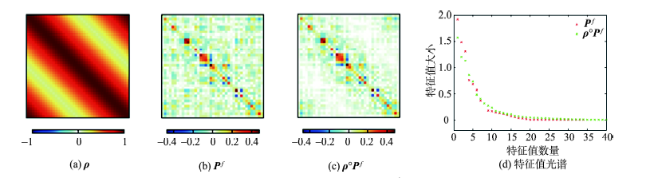
Fig.1 CL method′s impact on the background error covariance matrix Pf

图1 CL方法对背景误差协方差矩阵Pf的影响

4.2 近似协方差局地化方法(CL_new)对背景误差协方差矩阵的影响

CL方法不能直接用于ETKF,因此,探讨一种新的能应用于ETKF的近似协方差局地化方法,记为CL_new。为了考察CL_new方法对背景误差协方差矩阵 P f 的影响,在ETKF同化中,取 t = 10 时,CL_new局地化前后的 P f 作比较(图2)。其中, 图2(a)为状态变量间的相关系数矩阵 ρ ,图2(b)为CL_new局地化前的背景误差协方差矩阵 P f ,图2(c)为CL_new局地化后的背景误差协方差矩阵 P f ,图2(d)是CL_new局地化前后背景误差协方差矩阵 P f 的特征值光谱。
图2可知:(1)经过CL_new局地化后, P f 中截断距离以外的相关性未被消除,并且 P f 中协方差范围由之前的[-0.1,0.1]变为[-0.02,0.02],即相关系数的最大值减小了,如图2(c)所示,这表明CL_new方法不能消除背景误差协方差矩阵中的伪相关,只能系统地减小协方差的值;(2)经过CL_new局地化后, P f 的秩减小了,如图2(d)所示,这表明CL_new方法还降低了背景误差协方差矩阵的秩。综上可知,近似的协方差局地化方法(CL_new)不能消除伪相关,可能的原因是这种近似舒尔积减小了状态变量间的物理差异。
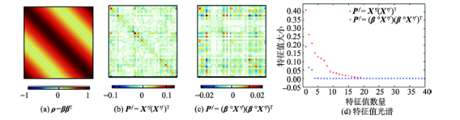
Fig.2 CL_new method’s impact on the background error covariance matrix Pf

图2 CL_new方法对背景误差协方差矩阵Pf的影响

4.3 CL_new方法和CL方法的近似程度

由上述可知,CL_new方法是一种局地化效果不太理想的近似CL方法。因此,考察CL_new方法和CL方法的近似程度,在ETKF同化中,取 t = 10 时,CL和CL_new局地化后的背景误差协方差矩阵作分析(图3)。其中,图3(a)为CL局地化后背景误差协方差矩阵 P f ,图3(b)为CL_new局地化后的背景误差协方差矩阵 P f ,图3(c)为CL和CL_new局地化后的背景误差协方差矩阵 P f 之差。
图3分析可知:(1)经过协方差局地化后, ( β β T ) ( X ' f ( X ' f ) T ) ( β X ' f ) ( β X ' f ) T 差异很大,如 图3(a)、(b)所示;(2)如图3(c)所示,单从主对角线上,二者差异很明显。综上表明, ( β β T ) ( X ' f ( X ' f ) T ) ( β X ' f ) ( β X ' f ) T 是一种不太精准的近似。
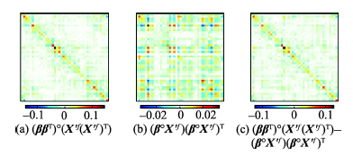
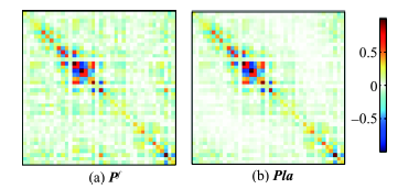
Fig.3 Approximation between CL_new and CL

图3 CL_new方法和CL方法的近似程度

4.4 局地分析方法(Local Analysis,LA)对背景 误差协方差矩阵的影响

由于CL_new方法消除伪相关的效果不明显,因此,寻求其他局地化方法用于ETKF同化。Sakov和韩培等[9,12]指出LA方法适用任何独立的同化方案,其原理是以待更新状态变量为中心,建立一个局地虚拟窗口,利用局地窗口内的观测,更新中心状态变量的背景误差协方差。
为了研究LA对ETKF同化的背景误差协方差矩阵的影响,在ETKF同化中,取 t = 10 时,LA局地化的背景误差协方差矩阵和未局地化的背景误差协方差矩阵作比较,结果如图4所示。图4(a)是第 i 个状态变量的裁剪系数矩阵FiFiT;图4(b)是未局地化的背景误差协方差矩阵,记为 P f ;图4(c)是第 i 个状态变量经LA局地化后的背景误差协方差矩阵,记为 Pla ( i ) 图4(c)中虚线框表示以第 i 个状态变量为中心的局地区域,实验中 i = 20 。为了更加清晰地对比未局地化和LA局地化对背景误差协方差矩阵的影响,本文给出了ETKF同化中 t = 10 时局地化后的全局背景误差协方差矩阵,如图5所示。其中,图5(a)是未局地化的全局背景误差协方差矩阵,记为 P f ;图5(b)LA局地化的全局背景误差协方差矩阵,记为 Pla
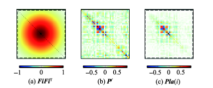
Fig.4 LA method′s impact on the background error covariance matrix

图4 LA对背景误差协方差矩阵的影响

图4、5可知:(1)LA方法可以消除背景误差协方差矩阵中的伪相关,减少远距离观测对待更新状态变量的影响;(2)相对于CL方法,LA方法每次只更新局地区域中心点的协方差,其他非中心元素的协方差不更新,即LA方法中背景误差协方差为异步更新,CL方法中背景误差协方差是同步更新。
Fig.5 Global background error covariance matrix

图5 全局背景误差协方差矩阵

4.5 不同局地化方法的ETKF同化效果

为了更清晰地分析各种局地化方法,本文比较了未局地化、协方差局地化方法(CL)、近似协方差局地化(CL_new)和LA的同化效果,如图6所示。其中,绿线表示ETKF未局地化(none)的同化效果,红线是ETKF近似协方差局地化(CL_new)的同化效果,蓝线是ETKF局地分析(LA)的同化效果,紫红线是EnKF协方差局地化(CL)的同化效果。
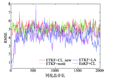
Fig.6 The data assimilation effects of different localization methods

图6 不同局地化方法的同化效果

由图(6)可知:(1)大体上,近似协方局地化(CL_new)的ETKF同化效果比未局地化的同化效果差,这表明:近似协方差局地化方法可适用于ETKF同化,但近似协方差局地化方法的同化结果误差较大,可能的原因是近似舒尔积 ( β β T ) ( X ' f ( X ' f ) T ) ( β X ' f ) ( β X ' f ) T 破坏了ETKF同化系统的动态平衡;(2)LA的ETKF同化效果比未局地化和CL_new方法的同化效果好,表明:LA方法可适用于ETKF同化,能获得较好的同化结果。(3)总体上,ETKF的LA同化效果比EnKF的CL同化效果好,但是由于CL不能直接用于ETKF同化,不能表明LA方法比CL方法好,因为同化效果是同化方案和局地化方法综合计算分析的结果。

5 结论

本文不仅在理论上详细分析了CL方法用于ETKF同化存在的问题,而且提出了一种近似CL方法(CL_new)。最后,结合Lorenz-96模型和ETKF方案,对近似CL方法的适用性进行实验验证和分析。实验结果表明:
(1)CL方法可消除背景误差协方差矩阵中的伪相关,减少远距离观测对待更新状态变量的影响;同时CL方法还可以增大背景误差协方差矩阵的秩。但是,CL方法不能直接用于ETKF同化。
(2)近似协方差局地化方法(CL_new)不能消除背景误差协方差矩阵中的伪相关;同时它还降低背景误差协方差矩阵的秩(不能增大有效的集合大小)。虽然近似协方差局地化方法可适用于ETKF同化,但其ETKF同化结果误差较大。其原因可能是近似舒尔积减小了状态变量间的物理差异,破坏了ETKF同化系统的动态平衡。
(3)LA方法能消除背景误差协方差矩阵中的伪相关,并且经过LA局地化后,ETKF的同化效果优于未局地化和近似协方差局地化。这表明LA方法可适用于ETKF同化,能获得较好的同化结果。

The authors have declared that no competing interests exist.

[1]
Kucukkaraca E, Fisher M.Use of analysis ensembles in estimating flow-dependent background error variances[M]. Reading, UK: European Centre for Medium-Range Weather Forecasts, 2006.

[2]
Sakov P, Oke P R.A deterministic formulation of the ensemble Kalman filter: an alternative to ensemble square root filters[J]. Tellus A, 2008,60(2):361-371.ABSTRACT The use of perturbed observations in the traditional ensemble Kalman filter (EnKF) results in a suboptimal filter behaviour, particularly for small ensembles. In this work, we propose a simple modification to the traditional EnKF that results in matching the analysed error covariance given by Kalman filter in cases when the correction is small; without perturbed observations. The proposed filter is based on the recognition that in the case of small corrections to the forecast the traditional EnKF without perturbed observations reduces the forecast error covariance by an amount that is nearly twice as large as that is needed to match Kalman filter. The analysis scheme works as follows: update the ensemble mean and the ensemble anomalies separately; update the mean using the standard analysis equation; update the anomalies with the same equation but half the Kalman gain. The proposed filter is shown to be a linear approximation to the ensemble square root filter (ESRF). Because of its deterministic character and its similarity to the traditional EnKF we call it the 鈥榙eterministic EnKF鈥, or the DEnKF. A number of numerical experiments to compare the performance of the DEnKF with both the EnKF and an ESRF using three small models are conducted. We show that the DEnKF performs almost as well as the ESRF and is a significant improvement over the EnKF. Therefore, the DEnKF combines the numerical effectiveness, simplicity and versatility of the EnKF with the performance of the ESRFs. Importantly, the DEnKF readily permits the use of the traditional Schur product-based localization schemes.

DOI

[3]
Whitaker J S, Hamill T M.Ensemble data assimilation without perturbed observations[J]. Monthly Weather Review, 2002,30(7):1913-1924.

[4]
Bishop C H, Etherton B J, Majumdar S J.Adaptive sampling with the ensemble transform Kalman filter. part i: theoretical aspects[J]. Monthly Weather Review, 2001,129(3):420-436.

[5]
Wang X, Bishop C H.A comparison of breeding and ensemble transform Kalman filter ensemble forecast schemes[J]. Journal of the Atmospheric Sciences, 2003,60(9):1140-1158.The ensemble transform Kalman filter (ETKF) ensemble forecast scheme is introduced and compared with both a simple and a masked breeding scheme. Instead of directly multiplying each forecast perturbation with a constant or regional rescaling factor as in the simple form of breeding and the masked breeding schemes, the ETKF transforms forecast perturbations into analysis perturbations by multiplying by a transformation matrix. This matrix is chosen to ensure that the ensemble-based analysis error covariance matrix would be equal to the true analysis error covariance if the covariance matrix of the raw forecast perturbations were equal to the true forecast error covariance matrix and the data assimilation scheme were optimal. For small ensembles (鈭100), the computational expense of the ETKF ensemble generation is only slightly greater than that of the masked breeding scheme. Version 3 of the Community Climate Model (CCM3) developed at National Center for Atmospheric Research (NCAR) is used to test and compare these ensemble generation schemes. The NCEP-NCAR reanalysis data for the boreal summer in 2000 are used for the initialization of the control forecast and the verifications of the ensemble forecasts. The ETKF and masked breeding ensemble variances at the analysis time show reasonable correspondences between variance and observational density. Examination of eigenvalue spectra of ensemble covariance matrices demonstrates that while the ETKF maintains comparable amounts of variance in all orthogonal and uncorrelated directions spanning its ensemble perturbation subspace, both breeding techniques maintain variance in few directions. The growth of the linear combination of ensemble perturbations that maximizes energy growth is computed for each of the ensemble subspaces. The ETKF maximal amplification is found to significantly exceed that of the breeding techniques. The ETKF ensemble mean has lower root-mean-square errors than the mean of the breeding ensemble. New methods to measure the precision of the ensemble-estimated forecast error variance are presented. All of the methods indicate that the ETKF estimates of forecast error variance are considerably more accurate than those of the breeding techniques.

DOI

[6]
Wei M, Toth Z, Wobus R, et al.Ensemble transform Kalman filter-based ensemble perturbations in an operational global prediction system at NCEP[J]. Tellus A, 2006,58(1):28-44.The initial perturbations used for the operational global ensemble prediction system of the National Centers for Environmental Prediction are generated through the breeding method with a regional rescaling mechanism. Limitations of the system include the use of a climatologically fixed estimate of the analysis error variance and the lack of an orthogonalization in the breeding procedure. The Ensemble Transform Kalman Filter (ETKF) method is a natural extension of the concept of breeding and, as shown by Wang and Bishop, can be used to generate ensemble perturbations that can potentially ameliorate these shortcomings. In the present paper, a spherical simplex 10-member ETKF ensemble, using the actual distribution and error characteristics of real-time observations and an innovation-based inflation, is tested and compared with a 5-pair breeding ensemble in an operational environment.

DOI

[7]
Evensen G.Data assimilation: the ensemble Kalman filter[M]. Berlin, Germany: Springer Science & Business Media, 2009.

[8]
Hamill T M, Whitaker J S, Snyder C.Distance-dependent filtering of background error covariance estimates in an ensemble Kalman filter[J]. Monthly Weather Review, 2001,129(11):2776-2790.

[9]
韩培,舒红,许剑辉.EnKF同化的背景误差协方差矩阵局地化对比研究[J].地球科学进展,2014,29(10):175-1185.在集合数据同化中,背景场误差的协方差估计特别重要。通常有限个成员的集合在估计背景误差协方差矩阵时会引入伪相关,从而造成协方差被低估、滤波发散。虽然协方差膨胀的经验性方法能一定程度缓解协方差被低估的问题,但不能消除协方差的伪相关问题。因此,结合EnKF方案探讨2种消除伪相关的局地化方法(协方差局地化方法和局地分析方法),分析这2种局地化方法对背景误差协方差矩阵、增益矩阵、集合转换矩阵以及同化结果的影响。实验结果表明:局地化方法不仅能消除背景误差协方差矩阵的伪相关,还可以增加背景误差协方差矩阵的秩;在"弱"同化强度下,2种局地化方法的增益矩阵和集合转换矩阵相等;随着同化强度的增大,增益矩阵和集合转换矩阵的差异会变大;在不同的同化强度下,2种局地化方法各具特色,相对而言,协方差局地化方法在更新集合均值和集合扰动上具有较强的鲁棒性。研究结论有助于背景场误差协方差的精细分析和估计。

DOI

[ Han P, Shu H, Xu J H.A comparative study of background error covariance localization in EnKF data assimilation[J]. Advances in Earth Science, 2014,29(10):1175-1185. ]

[10]
Hunt B R, Kostelich E J, Szunyogh I.Efficient data assimilation for spatiotemporal chaos: a local ensemble transform Kalman filter[J]. Physica D: Nonlinear Phenomena, 2007,230(1):112-126.Data assimilation is an iterative approach to the problem of estimating the state of a dynamical system using both current and past observations of the system together with a model for the system’s time evolution. Rather than solving the problem from scratch each time new observations become available, one uses the model to “forecast” the current state, using a prior state estimate (which incorporates information from past data) as the initial condition, then uses current data to correct the prior forecast to a current state estimate. This Bayesian approach is most effective when the uncertainty in both the observations and in the state estimate, as it evolves over time, are accurately quantified. In this article, we describe a practical method for data assimilation in large, spatiotemporally chaotic systems. The method is a type of “ensemble Kalman filter”, in which the state estimate and its approximate uncertainty are represented at any given time by an ensemble of system states. We discuss both the mathematical basis of this approach and its implementation; our primary emphasis is on ease of use and computational speed rather than improving accuracy over previously published approaches to ensemble Kalman filtering. We include some numerical results demonstrating the efficiency and accuracy of our implementation for assimilating real atmospheric data with the global forecast model used by the US National Weather Service.

DOI

[11]
Bergemann K, Reich S.A localization technique for ensemble Kalman filters[J]. Quarterly Journal of the Royal Meteorological Society, 2010,136(648):701-707.Ensemble Kalman filter techniques are widely used to assimilate observations into dynamical models. The phase space dimension is typically much larger than the number of ensemble members which leads to inaccurate results in the computed covariance matrices. These inaccuracies can lead, among other things, to spurious long range correlations which can be eliminated by Schur-product-based localization techniques. In this paper, we propose a new technique for implementing such localization techniques within the class of ensemble transform/square root Kalman filters. Our approach relies on a continuous embedding of the Kalman filter update for the ensemble members, i.e., we state an ordinary differential equation (ODE) whose solutions, over a unit time interval, are equivalent to the Kalman filter update. The ODE formulation forms a gradient system with the observations as a cost functional. Besides localization, the new ODE ensemble formulation should also find useful applications in the context of nonlinear observation operators and observations arriving continuously in time.

DOI

[12]
Sakov P, Bertino L.Relation between two common localisation methods for the EnKF[J]. Computational Geosciences, 2011,15(2):225-237.This study investigates the relation between two common localisation methods in ensemble Kalman filter (EnKF) systems: covariance localisation and local analysis. Both methods are popular in large-scale applications with the EnKF. The case of local observations with non-correlated errors is considered. Both methods are formulated in terms of tapering of ensemble anomalies, which provides a framework for their comparison. Based on analytical considerations and experimental evidence, we conclude that in practice the two methods should yield very similar results, so that the choice between them should be based on other criteria, such as numerical effectiveness and scalability.

DOI

[13]
Horn R A, Johnson C R.Matrix analysis[M]. Cambridge, UK: Cambridge University Press, 2012.

[14]
Schur J.Bemerkungen zur theorie der beschränkten bilinearformen mit unendlich vielen veränderlichen[J]. Journal Für Die Reine Und Angewandte Mathematik, 1911,140:1-28.

DOI

[15]
Petrie R.Localization in the ensemble Kalman filter[D]. Reading, UK: University of Reading, 2008.

[16]
Lorenz E N, Emanuel K A.Optimal sites for supplementary weather observations: simulation with a small model[J]. Journal of the Atmospheric Sciences, 1998,55(3):399-414.Anticipating the opportunity to make supplementary observations at locations that can depend upon the current weather situation, the question is posed as to what strategy should be adopted to select the locations, if the greatest improvement in analyses and forecasts is to be realized. To seek a preliminary answer, the authors introduce a model consisting of 40 ordinary differential equations, with the dependent variables representing values of some atmospheric quantity at 40 sites spaced equally about a latitude circle. The equations contain quadratic, linear, and constant terms representing advection, dissipation, and external forcing. Numerical integration indicates that small errors (differences between solutions) tend to double in about 2 days. Localized errors tend to spread eastward as they grow, encircling the globe after about 14 days.In the experiments presented, 20 consecutive sites lie over the ocean and 20 over land. A particular solution is chosen as the true weather. Every 6 h observations are made, consisting of the true weather plus small random errors, at every land site, and at one ocean site to be selected by the strategy being considered. An analysis is then made, consisting of observations where observations are made and previously made 6-h forecasts elsewhere. Forecasts are made for each site at ranges from 6 h to 10 days. In all forecasts, a slightly weakened external forcing is used to simulate the model error. This process continues for 5 years, and mean-square forecast errors at each site at each range are accumulated.Strategies that attempt to locate the site where the current analysis, as made without a supplementary observation, is most greatly in error are found to perform better than those that seek the oceanic site to which a chosen land site is most sensitive at a chosen range. Among the former are strategies based on the `breeding' method, a variant of singular vectors, and ensembles of `replicated' observations; the last of these outperforms the others. The authors speculate as to the applicability of these findings to models with more realistic dynamics or without extensive regions devoid of routine observations, and to the real world.

DOI

[17]
Gaspari G, Cohn S E.Construction of correlation functions in two and three dimensions[J]. Quarterly Journal of the Royal Meteorological Society, 1999,125(554):723-757.Abstract This article focuses on the construction, directly in physical space, of simply parametrized covariance functions for data-assimilation applications. A self-contained, rigorous mathematical summary of relevant topics from correlation theory is provided as a foundation for this construction. Covariance and correlation functions are defined, and common notions of homogeneity and isotropy are clarified. Classical results are stated, and proven where instructive. Included are smoothness properties relevant to multivariate statistical-analysis algorithms where wind/wind and wind/mass correlation models are obtained by differentiating the correlation model of a mass variable. the Convolution Theorem is introduced as the primary tool used to construct classes of covariance and cross-covariance functions on three-dimensional Euclidean space R 3 . Among these are classes of compactly supported functions that restrict to covariance and cross-covariance functions on the unit sphere S 2 , and that vanish identically on subsets of positive measure on S 2 . It is shown that these covariance and cross-covariance functions on S 2 , referred to as being space-limited , cannot be obtained using truncated spectral expansions. Compactly supported and space-limited covariance functions determine sparse covariance matrices when evaluated on a grid, thereby easing computational burdens in atmospheric data-analysis algorithms. Convolution integrals leading to practical examples of compactly supported covariance and cross-covariance functions on R 3 are reduced and evaluated. More specifically, suppose that gi and gj are radially symmetric functions defined on R 3 such that gi (x) = 0 for |x| > di and gj (x) = 0 for |xv > dj , O di + dj and |x - y| > 2 di , respectively, Additional covariance functions on R 3 are constructed using convolutions over the real numbers R , rather than R 3 . Families of compactly supported approximants to standard second- and third-order autoregressive functions are constructed as illustrative examples. Compactly supported covariance functions of the form C (x,y) := Co (|x - y|), x,y 鈭 R 3 , where the functions Co ( r ) for r 鈭 R are 5th-order piecewise rational functions, are also constructed. These functions are used to develop space-limited product covariance functions B (x, y) C (x, y), x, y 鈭 S 2 , approximating given covariance functions B (x, y) supported on all of S 2 脳 S 2 .

DOI

Outlines

/