
Journal of Geo-information Science >
Simulation and Analysis of Carbon Dioxide Concentration in the Surface Layer
Received date: 2015-12-30
Request revised date: 2016-05-11
Online published: 2017-02-17
Copyright
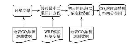
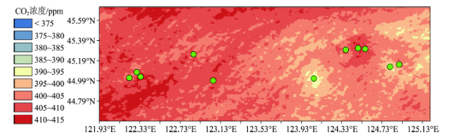
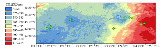
As an important cause of global warming, carbon dioxide concentration and its change has aroused worldwide concern. How to have an explicit understanding of the spatial and temporal distribution of carbon dioxide concentration is a crucial technical challenge for climate change research. In this paper, based on the in situ observation data set collected in the TanSat flight test area, the correlations between the carbon dioxide concentrations and the environmental variables are analyzed, and suitable environment variables can be selected to establish a regression equation, through which we obtain a preliminary trend of surface carbon dioxide concentrations. Then combining the multiple linear regression model and High Accuracy Surface Modelling (HASM), the carbon dioxide concentrations with a high accuracy in the entire test area are produced. The results indicate that the spatial distributions of the carbon dioxide concentrations in the study area are significantly different between three periods, and the short-wave radiation is an important factor for the regression equation. Because of the high temperature and drought condition, the highest concentration appears in the first period especially in the western area. The second period has a different distribution on the carbon dioxide concentration comparing with the previous period, as in this period the high value region moves eastward, and making the concentration high in the eastern area but low in the western area. Both of the second and third periods have similar characteristics except that the high value region in the eastern area is reduced in third period. Moreover, statistical analyses show that the mean absolute error and the mean relative error of the predicted value of the HASM model are 9.8 ppm and 2.48% respectively, which are both lower than the errors produced using the Kriging method, therefore the HASM model remains to have higher simulation accuracy in a condition of few sampling points and low sampling density. Therefore a combined method of multiple linear regression model and HASM model can be used as an effective method for simulating the spatial and temporal distribution of carbon dioxide concentration in the surface layer.
Key words: HASM method; carbon dioxide concentration; spatial simulation; WRF
LIU Yu , GUO Jianhong , YUE Tianxiang , ZHAO Na . Simulation and Analysis of Carbon Dioxide Concentration in the Surface Layer[J]. Journal of Geo-information Science, 2017 , 19(2) : 197 -204 . DOI: 10.3724/SP.J.1047.2017.00197
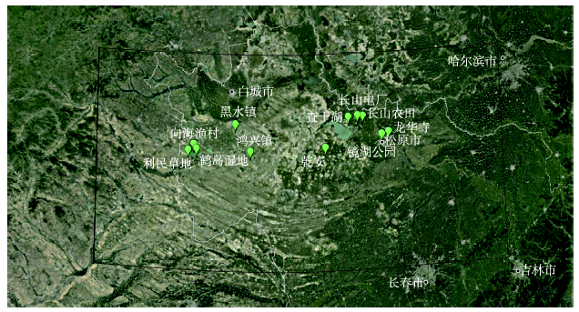
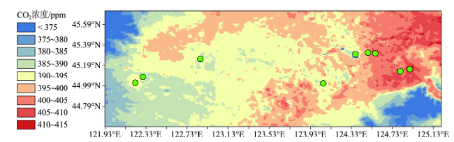
Fig.1 Location of automatic weather stations图1 自动气象站安置点分布图 |
Tab.1 Surrounding environment of automatic weather stations表1 自动气象站周边环境 |
| 气象站名称 | 植被状况 | 下垫面类型 |
|---|---|---|
| 镜湖公园 | 位于城区内,周围是附近居民开辟的小片菜地,植被高度较低,不远处就是成片的建筑物 | 城市 |
| 龙华寺 | 在一片果园中,植被高度较高约2 m。果树间隙种植了一些玉米 | 果园 |
| 长山农田 | 在大片农田中,植被覆盖度较高,植被高度约40 cm左右 | 农田 |
| 长山电厂 | 位于发电厂东侧约600 m,植被覆盖少,地表以裸土、石块、砖块为主。自动站北侧40 m外有大片农田,东侧有些闲置的砖堆 | 发电厂+农田 |
| 查干湖 | 距离查干湖约100 m,地表植被以杂草为主,植被高度很低 | 水体附近 |
| 乾安 | 位于一沙场内,自动站一侧是植被覆盖少的沙场,另一侧是植被覆盖多的杂草,杂草高度约40 cm左右 | 沙地+杂草 |
| 鸿兴镇 | 位于菜地中,自动站南侧主要是玉米等作物,其他区域为葱等高度较低的农作物 | 农田 |
| 黑水镇 | 位于荒地中,植被很少,主要是高度很矮的小丛的杂草,地表以裸土为主 | 裸土 |
| 鹤岛湿地 | 位于湿地,植被覆盖度较高,植被高度约1 m左右 | 湿地+草地 |
| 利民草地 | 位于大片草地中,植被覆盖度很高,植被高度约30 cm左右 | 草地 |
| 向海渔村 | 位于向海边的向日葵田中,向日葵约2 m | 水体附近 |
Fig.2 The flowchart of simulation图2 模拟流程图 |
Tab.2 Correlation analysis between CO2 concentration and environmental variables表2 各时段CO2浓度与环境变量相关性分析 |
| 时段 | |||
|---|---|---|---|
| 8月19日- 8月28日 | 8月29日- 9月7日 | 9月8日- 9月17日 | |
| 采样点数/个 | 11 | 10 | 9 |
| 纬度 | 0.1494 | -0.0185 | 0.1484 |
| 经度 | -0.2443 | 0.6686** | 0.5998* |
| 海拔 | 0.1884 | -0.4430 | -0.3562 |
| 雨量 | 0.0152 | 0.0247 | 0.0653 |
| 大气温度 | -0.1553 | -0.5578* | -0.4740* |
| 土壤温度 | -0.5031 | 0.0370 | 0.0678 |
| 向下短波辐射 | 0.6114** | -0.5739* | -0.1991 |
| 向上短波辐射 | 0.0322 | -0.6928** | -0.4077* |
| 土壤湿度 | 0.1407 | -0.2775 | -0.2722 |
| 大气湿度 | 0.2785 | 0.3789 | 0.2644 |
| 地表气压 | -0.1090 | 0.4328 | 0.4431* |
Tab.3 Regression models of CO2 concentration表3 CO2浓度回归方程 |
| 时段 | 回归方程 | 校正R2 | P |
|---|---|---|---|
| 8月19日-8月28日 | CO2= 327.995752+ 0.439485×向下短波辐射 | 0.304 | 0.046 |
| 8月29日-9月7日 | CO2= 682.554308-12.271210×2 m温度-0.833343×向上短波辐射 | 0.568 | 0.022 |
| 9月8日-9月17日 | CO2=-2714.532387-6.129403×2 m温度-0.510322×向上短波辐射+3.258770×地表气压 | 0.506 | 0.095 |
Fig.3 Spatial distribution of CO2 concentration from 19 August to 28 August图3 8月19日-8月28日CO2浓度空间分布模拟图 |
Fig.4 Spatial distribution of CO2 concentration from 29 August to 7 September图4 8月29日-9月7日CO2浓度空间分布模拟图 |
Fig.5 Spatial distribution of CO2 concentration from 8 September to 17 September图5 9月8日-9月17日CO2浓度空间分布模拟图 |
Tab.4 Absolute error and relative error between Kriging and HASM表4 Kriging与HASM误差分析 |
| 时段 | Kringing | HASM | |||
|---|---|---|---|---|---|
| MAE/ppm | MRE/% | MAE/ppm | MRE/% | ||
| 8月19日-8月28日 | 10.6 | 2.63 | 10.1 | 2.52 | |
| 8月29日-9月7日 | 11.3 | 2.89 | 10.7 | 2.74 | |
| 9月8日-9月17日 | 9.1 | 2.28 | 8.7 | 2.19 | |
| 平均 | 10.3 | 2.60 | 9.8 | 2.48 | |
The authors have declared that no competing interests exist.
| [1] |
[
|
| [2] |
|
| [3] |
|
| [4] |
IPCC. Climate change 2007: The physical science basis: contribution of working group I to the fourth assessment report of the Intergovernmental Panel on Climate Change[M]. Cambridge: Cambridge University Press, 2007.
|
| [5] |
|
| [6] |
|
| [7] |
[
|
| [8] |
|
| [9] |
Kuze, A, Suto, H, Nakajima, et al. Thermal and near infrared sensor for carbon observation Fourier-transform spectrometer on the greenhouse gases observing satellite for greenhouse gases monitoring[J]. Applied Optics, 2009,48:6716-6733.
|
| [10] |
|
| [11] |
[
|
| [12] |
|
| [13] |
|
| [14] |
|
| [15] |
|
| [16] |
|
| [17] |
[
|
| [18] |
|
| [19] |
|
| [20] |
[
|
| [21] |
[
|
| [22] |
[
|
| [23] |
[
|
| [24] |
|
| [25] |
[
|
| [26] |
[
|
| [27] |
|
| [28] |
[
|
| [29] |
[
|
/
| 〈 |
|
〉 |