Assessment of Polar Bear Habitats Stability from Remote Sensing

  • LI Haili ,
  • KE Changqing , *
Expand
  • School of Geographic and Oceanographic Sciences, Nanjing University, Nanjing 210023 China
*Corresponding author: KE Changqing, E-mail:

Received date: 2018-01-16

  Request revised date: 2018-06-13

  Online published: 2018-09-25

Supported by

National Key Research and Development Program of China, No.2018YFC1407203.

Copyright

《地球信息科学学报》编辑部 所有

Abstract

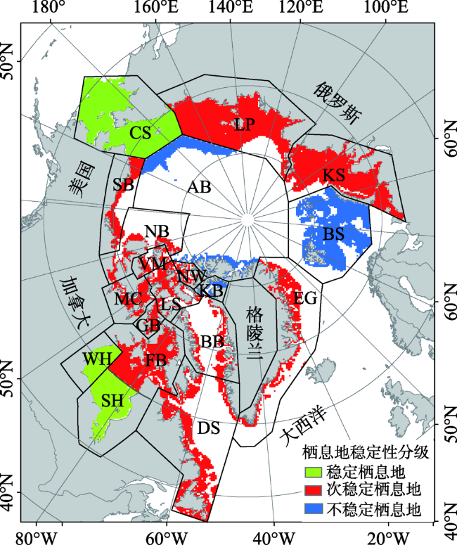
Polar bear is one of the most important mammals in the Arctic, but its number decreased in recent years. Polar bears are sensitive to changes of the sea ice distribution and depend on sea ice as a platform for hunting, moving and reproducing. In other words, sea ice is an important part of polar bear habitat. Climate is the main factor of sea ice changes. Therefore, it is very important to understand the current situation of polar bears as well as the effect of climate on the Arctic ecosystem. Although many researchers have devoted to find polar bears habitat using aerial survey in recent years, their methods require considerable human involvement and cannot be used to detect all habitats rapidly and effectively. Thus, it is necessary to find a method to quickly assess the polar bear habitat changes. Based on the sea ice concentration products from the United States National Snow and Ice Data Center (NSIDC) and the ETOPO1 bedrock product provided by the NOAA, the inter-annual variability of sea ice concentration, open water area, sea ice retreat, sea ice advance and the length of the open water season in the Arctic were analyzed. Then, the polar bear habitat stability were analized. The results indicate that from 1989 to 2016 the sea ice concentration has decreased, open water area increased and multiyear ice decreased. Most of the multiyear ice has converted to one-year ice. The sea ice appeared later and retreated earlier, so the length of the open water season increased significantly, an increase of 72 days compared to 1992. Barents Sea is the region with the most significant changes in open water area and the length of open water season among 19 habitats, with increasing rates of 9.71×10³ km2/a and 71.69 days/decade, respectively. Based on the change rates of the length of the open water season, we divide the polar bears habitats into three levels of conditions: stable, sub-stable and instable. The three stable habitats, including the Chukchi sea, Western Hudson Bay and Southern Hudson Bay are located in the lower latitudes compared with other habitats. There are 13 sub-stable habitats, including Laptev Sea, Kara Sea, East Greenland, Baffin Bay, Davis Strait, Foxe Basin, Gulf of Boothia, M’Clintock Channel, Viscount Melville, Norwegian Bay, Northern Beaufort Southern Beaufort and Lancaster Sound. The three unstable habitats are located in the north of 70°N, including Arctic Basin, Barents Sea and Kane Basin. Stable habitats are mainly in low latitudes, and unstable regions are all in high latitudes. The classification results show that the high latitude area is covered with more sea ice, but the inter-annual variation is very significant. In three unstable regions, polar bears have less time to adapt to the sea ice changes, and the inter-annual migration changes greatly, which is less favorable to the survival and development of polar bears.

Cite this article

LI Haili , KE Changqing . Assessment of Polar Bear Habitats Stability from Remote Sensing[J]. Journal of Geo-information Science, 2018 , 20(9) : 1327 -1337 . DOI: 10.12082/dqxxkx.2018.180057

1 引言

北极熊是生活在北极地区的标志性生物之一,是北极生物圈研究的重点对象,是一种能在恶劣环境下生存的生物[1,2]。有遥感观测资料以来,北极海冰不断减少[3,4,5,6,7],开阔水域面积持续增加。近十多年来,增加的速度大于过去的2倍[8],开阔水域季节长度变长[8,9,10]。海冰系统如此剧烈的变化对北半球的大气和海洋环流等造成很大影响[11]。不仅如此,海冰超过预期的缩减对北极生态系统也有很大的影响,小到北极的藻类、微生物,大到北极熊等高级哺乳动物[12,13,14]。北极熊主要依靠海冰进行狩猎、繁殖、活动等,海冰的减少给北极熊的生存带来巨大的威胁[15,16]。目前北极熊已经被列入《世界自然保护联盟》(IUCN, International Union for Conservation of Nature)濒危物种红色名录,定级为易危(VU, Vulnerability)生物[17]
过去北极熊栖息地主要根据人工野外调查来确定活动范围,利用生物标记的方法进行北极熊数量统计[18],这种方法耗费时间长,且受环境、危险性等因素的影响。当前,兴起了利用航空遥感手段来对北极熊进行研究,研究区大多集中在南哈得孙湾、西哈得孙湾和福克斯湾(北哈得孙湾),关注的重点是北极熊数量的变化[19,20]。该方法较传统方法在效率上有了很大的提升,但依旧不能快速实时地覆盖整个北极区域,适合中小尺度的北极熊研究。
PBSG (Polar Bear Specialist Group)根据地区划分了19个北极熊亚群[21],亦为19个北极熊栖息地。经估算目前北极熊所有亚群总和大约25 000头。研究表明北极熊正在变得消瘦[22]且数量在减少。北极熊以海豹为食,而海豹也是依赖于浮冰觅食、蜕皮、繁殖和休息,容易受到北极海冰变化的影响。因此海冰的减少导致食物的缺乏是北极熊减少的重要原因之一[23]。1980年加拿大西哈得孙湾雌性北极熊平均体重为650磅,2004年下降到507磅[24]。Lunn等[25]通过实时捕获和死亡数据估计哈得孙湾(西哈得孙湾、南哈得孙湾和福克斯湾)北极熊数量从1987年的1185只下降到2011年的806只。北极熊在夏季海冰大量消退前被迫去找寻和先前生活环境相似的栖息地,新栖息地的捕食环境或许并不能满足北极熊的生存,被迫改变捕食习惯,甚至食用青草等素食[26]。北极19个栖息地中7个栖息地出现数量下降趋势,其中西哈得孙湾和南波弗特两个栖息地北极熊数量减少已经确信是气候变化导致海冰减少引发的结果,4个基本稳定,一个可能在增加[27,28,29]。随着对海冰与北极熊栖息地关系的了解,许多学者开始寻求找到一个海冰指标来量化19个栖息地活动范围的变化。海冰密集度是最直接的海冰参数,Rode等直接把它作为栖息地度量因子[30]。后续又发展了春季融冰期或秋季结冰期[31,32,33,34]、无冰期或覆冰期长度[35,36]、春季海冰消退时间、秋季海冰出现时间、海冰覆盖天数[37]等度量参数。Stern[37]提出的几个海冰指标被PBSG所采用。目前虽然提出较多海冰指标,但是缺乏综合性、实际性考量。如海冰密集度指标它只表示了海冰空间上的占比,海冰密集度大,只能表明该区域海冰面积占比大,但没有指明哪部分是海冰。Stern[37]认为海冰最小面积出现在9月,最大面积出现在3月来计算相应的海冰度量指标,忽视了气候变暖,海冰最小、最大面积时间变化的现状。因此需要一个统一、综合且自动性高的标准来对栖息地进行度量,进而对北极熊栖息地进行稳定性等级划分。
海冰融化成开阔水域之后,北极熊生活区域减小,被迫发生转移,转移的时间与海冰消退时间和出现时间有关,北极熊在某个区域生活时间的长短与开阔水域季节长度密切相关。利用开阔水域季节长度变化率,可以有效地反映北极熊19个栖息地的海冰-海水变化情况。开阔水域季节长度变化率越大,表明该区域越不稳定,未来不适合继续成为北极熊狩猎和活动的区域。因此,求解开阔水域季节长度变化率来度量北极熊栖息地变化情况,使评价北极熊栖息地稳定性和判断北极熊数量变化趋势简单易行,对评估未来北极熊数量与种群分布有重要意义,可以为人类保护北极熊这种濒危物种提供数据支持和决策参考。不仅如此,该度量方法除了可以应用在北极熊上,也可以适当推广到其他依赖海冰为栖息地的高食物链生物上,如海豹等,具有重要的现实意义。
本文提出一种基于海冰密集度数据的开阔水域季节长度变化率来度量北极熊栖息地范围变化情况。基于ETOPO1全球地形高程数据将水深小于300 m的区域筛选出来,作为栖息地中北极熊海上主要活动区域[37]。结合2种数据得出开阔水域面积,开阔水域季节长度,最终得出本文的海冰度量指标——开阔水域季节长度变化率。这种方法能够快速得出北极熊栖息地的变化现状以及发展趋势。

2 数据源与研究方法

2.1 研究区概况

研究区为PBSG划分的北极熊19个栖息地 (图1),中英文对照见表1。19个栖息地均位于北半球较高纬度区域,各区域内均有一定的海冰覆盖,纬度越高,海冰覆盖越广。其中的13个栖息地部分或全部位于加拿大境内。研究区除了有北极熊的分布之外,还生活着北极狐、北极海象、北极狼、鲸等生物,生物多样性丰富。
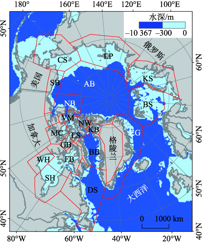
Fig.1 Location and water depth of the 19 polar bear habitats

图1 19个北极熊栖息地及水深分布

Tab.1 Habitats in English and Chinese

表1 栖息地中英文对照

序号 英文全称 英文简写 中文名称 序号 英文全称 英文简写 中文名称
1 Kane Basin KB 凯恩盆地 11 Western Hudson Bay WH 西哈得孙湾
2 Baffin Bay BB 巴芬湾 12 Southern Hudson Bay SH 南哈得孙湾
3 Lancaster Sound LS 兰开斯特海峡 13 Davis Strait DS 戴维斯海峡
4 Norwegian Bay NW 挪威湾 14 East Greenland EG 东格陵兰
5 Viscount Melville VM 梅尔维尔子爵海峡 15 Barents Sea BS 巴伦支海
6 Northern Beaufort NB 北波弗特 16 Kara Sea KS 喀拉海
7 Southern Beaufort SB 南波弗特 17 Laptev Sea LP 拉普捷夫海
8 M’Clintock Channel MC 麦克林托克海峡 18 Chukchi Sea CS 楚科奇海
9 Gulf of Boothia GB 布西亚湾 19 Arctic Basin AB 北极盆地
10 Foxe Basin FB 福克斯湾

2.2 数据源

2.2.1 海冰密集度
海冰密集度是指一个海区内海冰面积所占百分比[38],数据来自美国雪冰数据中心(NSIDC)的Sea Ice Concentrations from Nimbus-7 SMMR DMSP SSM/I-SSMIS Passive Microwave Data和Near-Real-Time DMSP SSMIS Daily Polar Gridded Sea Ice Concentrations产品(http://nsidc.org/data)。第一个产品选择1989年1月到2014年12月的数据,第二个产品选择2015年1月到2016年12月的数据。采用NASA戈达德空间飞行中心水循环实验室的NASA Team 算法[39,40]进行反演,来获取海冰相关参数。数据覆盖整个北极,空间分辨率为 25 km×25 km,时间分辨率为每日一次,TIF格式,北极方位投影。
2.2.2 ETOPO1全球地形高程数据
ETOPO1全球地形高程数据由NGDC美国地球物理中心发布,可从NOAA下载获得(http://www.ngdc.noaa.gov/mgg/global/global.html)。ETOPO1结合了陆地地形和海洋深度测量,由全球和区域数据集组成。目前有冰表面和基岩两类产品,冰表面产品相对于基岩产品不同的地方在于南极和格陵兰2个区域,其他区域数值是一样的,基岩产品是从水底算到冰盖底部,而冰表面产品则是加上了冰盖的厚度。本文采用基岩产品中的海洋水深数据,原始数据为FLT格式,空间分辨率为1弧分。

2.3 研究方法

2.3.1 预处理方法
从美国雪冰中心下载的海冰密集度产品为0-255灰度值数据。其中254代表大陆;253代表大陆轮廓、海岸线;251是极点附近的数据缺失空洞,假设该数据空洞的海冰密集度为100%。首先提取出大陆和大陆轮廓,再将其余所有像元值除以251将灰度值转换为0-100%[41],用以表示海冰密集度。
将ETOPO1原始数据定义为WGS_1984地理坐标系,并进行极地方位投影变换,再将变换后的数据进行栅格转换,获得地形高程栅格数据。将上述地形高程栅格数据的空间分辨率重采样至与海冰密集度数据相同的分辨率,即25 km×25 km。
2.3.2 开阔水域面积和季节长度
计算开阔水域面积公式如下:
W = 100 % - SIC × S (1)
式中:W表示栖息地开阔水域面积;S栅格表示开阔水域像元的栅格面积;SIC表示海冰密集度;海冰外缘线面积是影像中海冰密集度大于等于15%的所有栅格像元面积的总和。将海冰密集度大于等于15%的每个栅格的面积乘以对应栅格的海冰密集度,最后再累加得到的面积为海冰面积[41]。由海冰面积的求法可推开阔水域面积求法。100%减去SIC得到开阔水域百分比,将开阔水域百分比与S栅格相乘得到单个像元开阔水域面积,最后将每个栖息地内开阔水域像元的开阔水域面积累加得到该栖息地的W[8]。由每一年开阔水域面积最大值与最小值相减求得年平均变化量,再根据年平均变化量求得多年平均变化量B。然后由开阔水域面积最小值多年平均(A)和多年平均变化量得到判断海冰消退时间和出现时间的阈值Z[10]。当开阔水域面积高于判断阈值Z时对应的日期记为当年海冰消退时间,当开阔水域面积低于判断阈值Z时对应的日期为海冰出现时间。海冰出现时间与海冰消退时间的差值,即开阔水域季节长度。确定海冰消退和出现时间的判断阈值Z[10]的公式如下:
Z = A + K × B (2)
式中:K为调节系数,取值范围为[0.4,0.6],K的最佳取值为0.5[10]
2.3.3 方法流程
对海冰密集度和ETOPO1数据经过相应预处理,获得符合海冰密集度和水深要求的目标像元,得到开阔水域面积和季节长度后,最终获得开阔水域季节长度变化率(图2)。
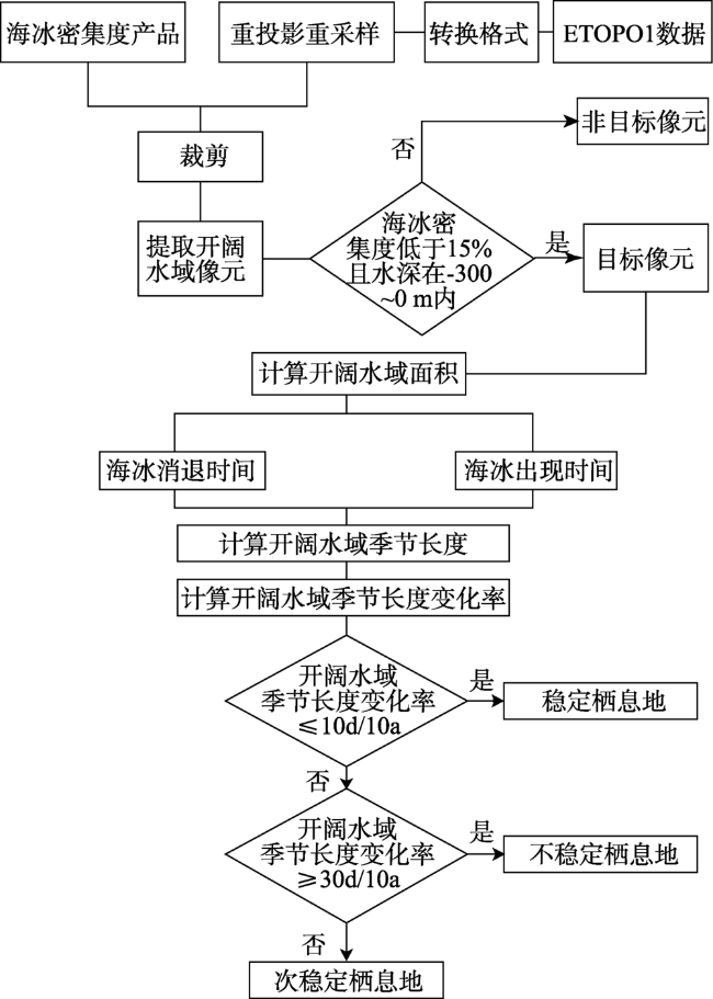
Fig. 2 Flowchart for determining the stability of the polar bear habitat

图2 北极熊栖息地稳定性判断流程图

3 结果与讨论

3.1 海冰密集度

2016年海冰面积达到有遥感观测数据以来的最低值。海冰变化有明显的季节特征,3月海冰密集度最高,高值区像元占较大比例。9月海冰密集度下降到最小值,海冰覆盖范围达到一年的最小值(图3),是北极熊活动最受限制的时期。选取海冰密集度最小的9月作出每隔3年的海冰密集度变化图,得出海冰密集度呈现降低的趋势,2007年是海冰覆盖最小的一年,而2016年是海冰高密度值占比最小的一年(图4)。喀拉海1989年9月将近1/3的区域有高密集度的海冰覆盖,2007年以后,9月基本不再有海冰覆盖。北极盆地1989年9月几乎全境都有海冰覆盖,最近几年始终存在部分区域不再有海冰覆盖。多年冰大量减少,变为一年冰。
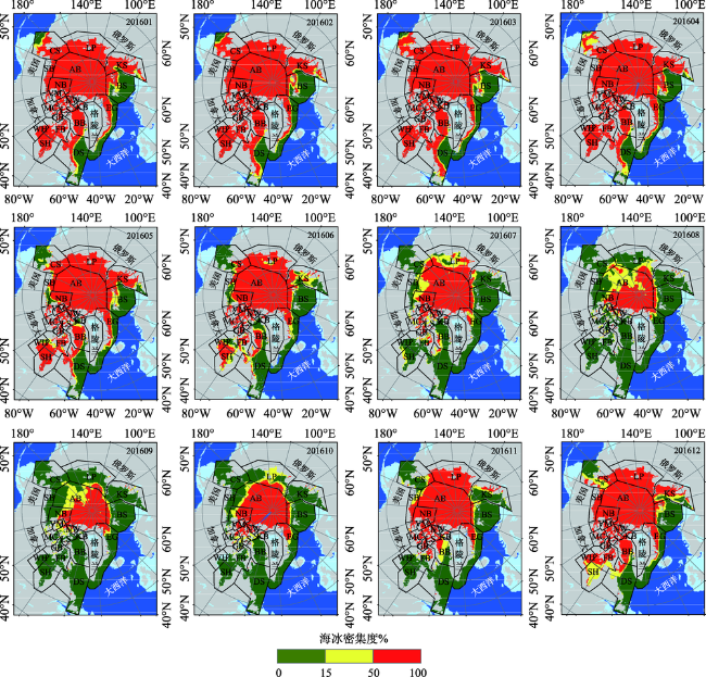
Fig. 3 Monthly variation of sea ice concentration in 2016

图3 2016年海冰密集度月变化

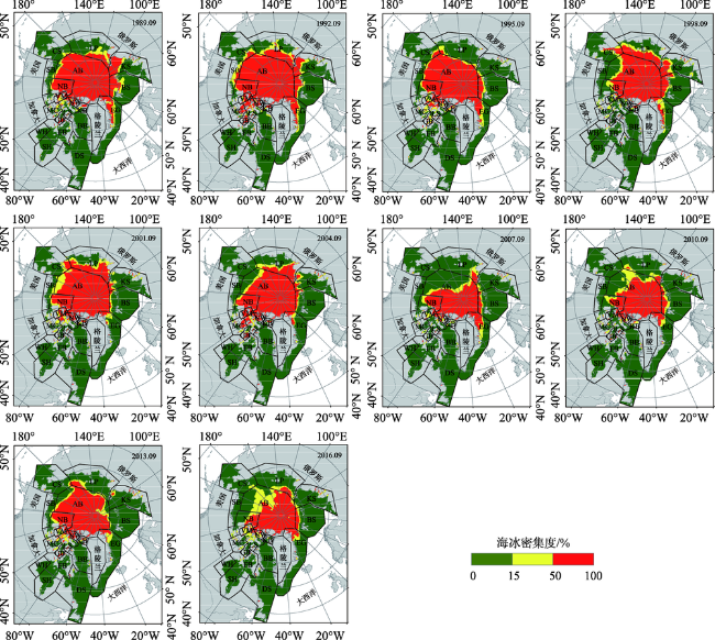
Fig. 4 Sea ice concentration in September from 1989 to 2016

图4 1989-2016年9月海冰密集度变化

3.2 开阔水域

3.2.1 开阔水域面积
以2001年为分段点[8],对整个研究区开阔水域面积变化进行分段分析。开阔水域总面积呈现年际波动、整体增加的趋势,速度为30.29×10³ km2/a,2016年达到有遥感观测资料以来的最大值。2001年以来,增加速度大幅提升,接近1989-2001年的2倍,分别为17.83×103 km2/a和33.66×103 km2/a(图5)。
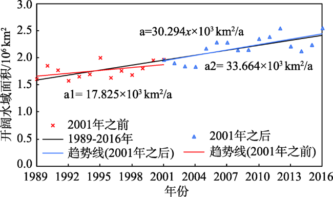
Fig. 5 The annual change of open water area and subparagraph of its slope in North polar region

图5 北极开阔水域面积变化及斜率分段

凯恩盆地、布西亚湾、梅尔维尔子爵海峡、挪威湾这4个栖息地开阔水域很少,是海冰常年覆盖区域。北极盆地是所有栖息地中所处纬度最高、面积较大的区域,自2006年开始,每年都有开阔水域分布且面积持续增多。喀拉海、巴伦支海是开阔水域面积增加最显著的2个区域,增长速度分别为 6.48×10³ km2/a和9.71×103 km2/a。变化最无规律的是拉普捷夫海,开阔水域面积先经历了大幅下降,后又迅速增加(图6)。
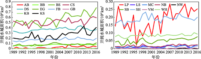
Fig. 6 The annual change of open water area in the 19 polar bear habitats

图6 19个北极熊栖息地开阔水域面积变化

3.2.2 开阔水域季节长度
北极海冰消退时间介于6-7月之间,随着年份的推移,海冰消退时间不断提前,由7月提前到6月。海冰出现时间介于10-12月,近20多年来海冰出现时间不断延后,从10月推迟到12月。2016年海冰消退时间相较于海冰消退最晚的1992年提前了27 d,提前速度为7.52 d/10 a。海冰出现时间相较于海冰出现最早的1992年推迟了45 d,时间为12月7日,打破了有遥感记录以来海冰最晚出现的记录,延迟速度为12.07 d/10 a(图7(a))。开阔水域季节长度同开阔水域面积变化相似,呈现年际波动,总体增加的趋势。2016年开阔水域季节长度相较于最低值1992年增加了72 d,增加速度为 19.59d/10 a(图7(b))。
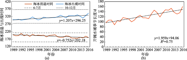
Fig. 7 The day of the year (DOY) of the initial sea ice retreat and advance and the length of the open water season in the North Polar region

图7 北极海冰消退、出现时间和开阔水域季节长度

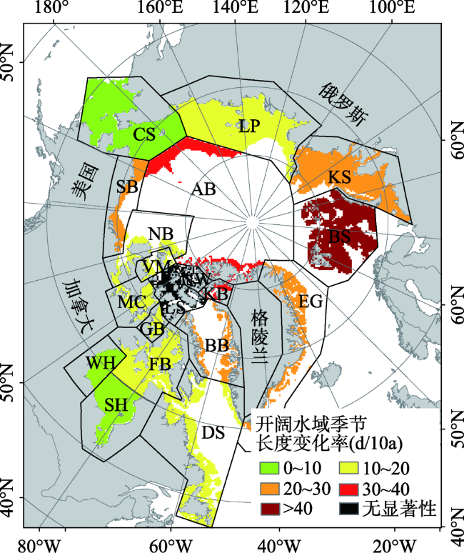
Fig. 8 Changing rate of the length of the open water season for polar bear habitat

图8 北极熊栖息地开阔水域季节长度变化率

在所有北极熊栖息地中,戴维斯海峡开阔水域季节长度最长,达到202 d,超过1/3的时间是属于开阔水域占主导。挪威湾是其中开阔水域季节长度最短的栖息地,约13 d,为海冰主导的区域。季节长度变化最快的有喀拉海、凯恩海湾和北极盆地,增长速度为71.69 d/10a、33.84 d/10a和31.88 d/10a(表2),海冰年代际变化剧烈,减少显著(0.01显著性水平)。除了挪威湾和兰开斯特海峡,其余区域均通过显著性水平检验,变化趋势显著。挪威湾开阔水域季节长度变化率非常小,但是年际变化非常大,1989年以来先经历了大幅度的减少,后又持续增加。兰开斯特海峡开阔水域季节长度年际变化波动较大,变化趋势不显著。
Tab. 2 The length of the open water season and its change rate in 19 polar bear habitats

表2 19个北极熊栖息地开阔水域季节长度及变化率

栖息地 均值/d 标准差/d 变化率/(d/10a) 可决系数R2
AB 48.25 35.84 31.88 0.54**
BB 163.93 32.23 24.94 0.41**
BS 174.79 79.52 71.69 0.55**
CS 176.39 16.42 9.81 0.24**
DS 202.00 23.46 14.83 0.27**
EG 84.14 34.56 24.74 0.35**
FB 135.68 17.50 11.54 0.27**
GB 40.50 25.03 13.51 0.20*
KB 33.75 36.88 33.84 0.57**
KS 104.36 29.91 24.54 0.46**
LP 70.57 25.01 14.04 0.21*
LS 35.54 25.55 9.66 0.10
MC 50.21 24.30 12.76 0.19*
NB 95.71 26.82 14.00 0.18*
NW 13.29 19.61 0.74 0.00
SB 94.18 28.64 22.31 0.41**
SH 152.32 16.37 7.72 0.15*
VM 22.00 23.57 14.64 0.26**
WH 149.43 15.96 9.38 0.23**

注:*在0.05水平上显著相关;**在0.01水平上显著相关

3.2.3 北极熊栖息地稳定性度量指标
将每10年开阔水域季节长度变化率反映在空间分布上,以10、20、30和40为间隔进行划分。共 5个栖息地开阔水域季节长度变化率低于10 d/10a,但是挪威湾和兰开斯特海峡没有通过显著性检验,线性回归得到的曲线不能反映真实变化的结果,归为无显著性类。7个栖息地位于10-20的区间,巴芬湾、东格陵兰、喀拉海和南波弗特分布在20-30的区间,北极盆地和凯恩盆地位于30-40的区间,巴伦支海超过了40 d/10 a。该指标最早被stern[37]在其文章中采用,现在被PBSG纳为衡量亚群变化的海冰参数之一。Stern等将计算开阔水域季节长度的海冰消退时间定义为海冰面积在达到夏季最小值的过程中,海冰面积减少到低于某一特定的阈值的时间。海冰出现时间则是海冰面积升高到超过该阈值的时间。阈值的计算方法是先计算1979-2014年3月和9月的平均海冰面积,两者差值的绝对值加上3月平均海冰面积。然后海冰出现时间和消退时间作差得到开阔水域季节长度。是基于海冰面积最大值出现在3月,海冰面积最小值出现在9月来计算的。但随着气候变暖加剧,海冰面积最小值出现时间在延后,最大值出现时间在提前。本文采用Arrigo等[10]的定义方法,更符合海冰变化的真实情况。
虽然方法有所差异,但本文得到的结果与Stern等[36]得到的结果基本一致,即巴伦支海变化是最显著的,其次是北极盆地,且符合19个栖息地实际海冰变化情况,能够真实反映北极熊生活区域的海冰变化以及未来栖息地的发展趋势。
3.2.4 北极熊栖息地稳定性评估结果
将开阔水域季节长度变化率低于10 d/10a的栖息地划分为稳定栖息地,10 d/10a到30 d/10a的栖息地归为次稳定栖息地,将大于30 d/10a的栖息地归为不稳定栖息地。挪威海和兰开斯特海峡的开阔水域季节长度变化率小于10 d/10a,但是开阔水域季节长度年际波动大,变化趋势不显著,于是将其降一个等级归为次稳定栖息地。位于高纬度的北极盆地、巴伦支海和凯恩盆地均属于不稳定区域(图9),海冰减少显著,按照该发展速度,对北极熊的生存极其不利,北极熊迁移更加频繁,适应新环境的时间大大减少,北极熊可能会因其生活的区域变化太大,对其生命造成威胁。位于较高纬度的拉普捷夫海、喀拉海、东格陵兰等13个亚群区属于次稳定区(图9)。楚科奇海、西哈得孙湾和南哈得孙湾均位于栖息地中的较低纬度,为稳定栖息地,开阔水域季节长度增加缓慢,海冰变化小,北极熊生境较为稳定。Lunn等[24]曾对西哈得孙湾的北极熊数量进行估计,1985年以来其数量在缓慢减少,2000年以来数量基本保持稳定,证明西哈得孙湾划分是正确的。Obbard等[20]基于航空测量估计南哈得孙湾北极熊的丰度,得出从1986年以来,北极熊数量没有显著的变化,这与本文将其划为稳定栖息地相吻合。以上分类结果可为未来几年内北极熊分布作出预测。当前属于稳定区的栖息地,纬度低,气温相对较高。3个亚群区开阔水域季节长度均超过140 d,若气温持续升高,海冰持续减少,则未来可能出现一整年海冰不存在的情况,那给北极熊带来的后果将是致命的。对于长期而言,如海冰减少的背景不能改变,整个北极将可能不再适合北极熊生活,北极熊数量将持续快速减少,遭受灭绝的威胁。
Fig.9 Stability assessment result for the habitats

图9 北极熊栖息地稳定性评估结果

4 结论

本文基于美国雪冰中心的海冰密集度和NOAA的ETOPO1数据,计算开阔水域面积、海冰消退时间、海冰出现时间和开阔水域季节长度,从而得到开阔水域季节长度变化率,以此为依据来评估北极熊栖息地稳定性,得到以下结论:
(1)北极海冰密集度在9月达到最低,年际间呈现降低的趋势。开阔水域总面积呈现年际波动、整体增加的趋势。海冰消退时间不断提前,出现时间不断延后,导致开阔水域季节长度大幅增加。巴伦支海是所有栖息地中开阔水域面积和季节长度增加贡献最大的海域,变化速度分别为9.71×10³ km2/a和71.69 d/10a。
(2)将开阔水域季节长度变化率作为评估北极熊栖息地稳定性的度量指标,得出目前大多数北极熊分布的区域为次稳定栖息地。不稳定栖息地均位于70°N以北。稳定栖息地基本位于70°N以南。高纬度栖息地海冰减少显著,年际变化大,对北极熊生活造成的影响将大于较低纬度地区。低纬度栖息地变化比较稳定,北极熊在这些区域有更长的适应时间。
(3)该评估结果可为短期几年或十几年内北极熊分布作出预测,但是对于未来几十年甚至上百年来说,若海冰减少的现状没有改变,甚至速度越来越快的背景下,即使是目前稳定的栖息地也将不再适合北极熊生活,必须引起人们的重视。随着遥感技术在空间分辨率和时间分辨率的进一步提高,以及北极科考的进一步推进,会有更多、更精确的实测资料和遥感数据来为北极熊的分布、数量和栖息地的增加或消失进行评估和验证。未来可利用更高精度的遥感影像来尝试提取北极熊的分布位置,不仅能够分析现有19个栖息地的稳定情况,为评价栖息地稳定性的指标提供进一步的验证。还能得出栖息地位置的改变,判断栖息地的迁移变化。

The authors have declared that no competing interests exist.

[1]
高登义. 北极之王北极熊[J].城市与减灾,2006(6):54-63.北极熊与浮冰的关系 在北极地区,北极熊主要生活在北冰洋的浮冰区。生物学家统计发现,在北冰洋,哪儿浮冰多,哪儿的北极熊也多。原因之一,北极熊是肉食动物,主要猎食海豹和 海象,而海豹和海象常常生活在浮冰区,海象喜欢群居在浮冰上,海豹喜欢躺在浮冰上休息、晒太阳;原因之二,北极熊不善潜冰,海豹和海象却是水下潜泳的健 将,北极熊要猎食海豹和海象也只有在浮冰上的可能性最大。

DOI

[ Gao D Y.King of the North Pole: Polar bear[J]. City and Disaster Reduction, 2006(6):54-63. ]

[2]
Derocher A E.Polar Bears[M]. Baltimore: The Johns Hopkins University Press, 2012.

[3]
Cavalieri D J, Parkinson C L, Vinnikov K Y.30-year satellite record reveals contrasting Arctic and Antarctic decadal sea ice variability[J]. Geophysical Research Letters, 2003,30(18):1-4.

[4]
柯长青,彭海涛,孙波,等.2002年-2011年北极海冰时空变化分析[J].遥感学报,2013,17(2):452-466.基于2002年-2011年AMSR-E海冰密集度数据, 分析了北极海冰的时空变化特征及其原因。结果表明海冰外缘线面积每年减小8.28×10<sup>4</sup> km<sup>2</sup> 下降趋势最快的季节为夏季, 下降速度是1979年-2006年的两倍多, 而且海冰密集度也在降低。2003年、2004年的冰情相对较重, 2007年海冰面积最小。长期冰在2002年-2010年间减少了近30%, 减少的区域主要在波弗特海、楚科奇海、东西伯利亚海、拉普贴夫海、喀拉海以及由这些边缘海向北极方向延伸的北冰洋的广大区域, 长期冰减少的地方大部分为季节性海冰增加的地方。海冰面积与年平均气温之间有显著的负相关关系, 随着全球气候变暖的加剧, 这种减小趋势将会持续。

DOI

[ Ke C Q, Peng H T, Sun B, et al.Spatio-temporal variability of Arctic sea ice from 2002 to 2011[J]. Journal of Remote Sensing, 2013,17(2):452-466. ]

[5]
Kinnard C, Zdanowicz C M, Fisher D A, et al.Climatic analysis of sea-ice variability in the Canadian Arctic from operational charts,1980-2004[J]. Annals of Glaciology, 2006,44(1):391-402.

DOI

[6]
Stroeve J, Holland M M, Meier W, et al.Arctic sea ice decline: Faster than forecast[J]. Geophysical research letters, 2007,34(9):529-536.From 1953 to 2006, Arctic sea ice extent at the end of the melt season in September has declined sharply. All models participating in the Intergovernmental Panel on Climate Change Fourth Assessment Report (IPCC AR4) show declining Arctic ice cover over this period. However, depending on the time window for analysis, none or very few individual model simulations show trends comparable to observations. If the multi-model ensemble mean time series provides a true representation of forced change by greenhouse gas (GHG) loading, 33-38% of the observed September trend from 1953-2006 is externally forced, growing to 47-57% from 1979-2006. Given evidence that as a group, the models underestimate the GHG response, the externally forced component may be larger. While both observed and modeled Antarctic winter trends are small, comparisons for summer are confounded by generally poor model performance.

DOI

[7]
Dong H J, Zou X L.Variations of sea ice in the Antarctic and Arctic from 1997 to 2006[J]. Frontiers of earth science, 2014,8(3):385-392.Sea ice in polar areas is an important part of the global climate system. In order to obtain variations in sea ice extent for the Antarctic and Arctic, this paper analyzed the Special Sensor Microwave/Imager (SSM/I) sea ice data product dating from March 1, 1997 to December 31, 2006. During this period, the sea ice extent increased in the Antarctic with the trend of (0.5467±0.4933)×10 4 km 2 ·yr 611 , and decreased in the Arctic with the trend of (617.6125±0.3503)×10 4 km 2 ·yr 611 . In different sectors of the Antarctic, variations of the sea ice extent are different. The sea ice extent increased in the Weddell Sea and Indian Ocean, but decreased in the Ross Sea, Western Pacific Ocean, and Bellingshausen/Amundsen Seas.

DOI

[8]
李海丽,柯长青.1982-2016年北极开阔水域变化[J].海洋学报,2017,39(12):109-121.

[ Li H L, Ke C Q.Open water variability in the North Pole from 1982 to 2016[J]. Acta Oceanologica Sinica, 2017,39(12):109-121. ]

[9]
Pabi S, Dijken G L V, Arrigo K R. Primary production in the Arctic Ocean, 1998-2006[J]. Journal of Geophysical Research, 2008,113(C8):185-198.1] Sea ice in the Arctic Ocean has undergone an unprecedented reduction in area and thickness in the last decade, exposing an ever increasing fraction of the sea surface to solar radiation and increasing the habitat suitable for phytoplankton growth. Here we use a primary production algorithm that utilizes remotely sensed chlorophyll a, sea surface temperature, and sea ice extent data to quantify interannual changes in phytoplankton production in the Arctic Ocean between 1998 and 2006. Our results show that since 1998, open water area in the Arctic has increased at the rate of 0.07 0103 106 km2 a0908081 (where a is years), with the greatest increases in the Barents, Kara, and Siberian sectors, particularly over the continental shelf. Although pan-Arctic primary production averaged 419 00± 33 Tg C a0908081 during 19980900092006, recent increases in open water area have lead to higher rates of annual production, which reached a 9-year peak in 2006. Annual production was roughly equally distributed between pelagic waters (less productive but greater area) and waters located over the continental shelf (more productive but smaller area). Interannual differences are most tightly linked to changes in sea ice extent, with changes in sea surface temperature (related to the Arctic Oscillation) and incident irradiance playing minor roles. Estimation of primary production in the Arctic will aid the assessment of air-sea CO2 fluxes and improve our understanding of the ecological and biogeochemical changes that could take place if ice cover continues to decrease.

DOI

[10]
Arrigo K R, Dijken G L V. Secular trends in Arctic Ocean net primary production[J]. Journal of Geophysical Research, 2011,116(C9):1527-1540.1] A satellite-based study was conducted to document daily changes in net primary production (NPP) by phytoplankton in the Arctic Ocean from 1998 to 2009 using fields of sea ice extent, sea surface temperature, and chlorophyll a concentrations. Total annual NPP over the Arctic Ocean exhibited a statistically significant 20% increase between 1998 and 2009 (range = 441090009585 Tg C yr0908081), due mainly to secular increases in both the extent of open water (+27%) and the duration of the open water season (+45 days). Increases in NPP over the 12 year study period were largest in the eastern Arctic Ocean, most notably in the Kara (+70%) and Siberian (+135%) sectors. NPP per unit area for the Arctic Ocean averaged 101 g C m0908082 yr0908081 with no significant change over the study period. In the western sectors, NPP ranged from 71.3 00± 11.0 g C m0908082 yr0908081 in the Beaufort to 96.9 00± 7.4 g C m0908082 yr0908081 in the Chukchi, while in the more productive eastern Arctic, annual NPP between 1998 and 2009 ranged from 101 00± 15.8 in the Siberian sector to 121 00± 20.2 in the Laptev. Results of a statistical analysis suggest that between 1979 and 1998 (prior to the launch of SeaWiFS and MODIS), total Arctic NPP likely averaged 438 00± 21.5 Tg C yr0908081. Moreover, when summer minimum ice cover drops to zero sometime during the first half of this century, annual NPP in the Arctic Ocean could reach 090804730 Tg C yr0908081. Nutrient fluxes into Arctic surface waters need to be better understood to determine if these projected increases are sustainable.

DOI

[11]
Aagaard K, Carmack E C.The role of sea ice and other fresh water in the Arctic circulation[J]. Journal of Geophysical Research: Oceans, 1989,94(C10):14485-14498.Salinity stratification is critical to the vertical circulation of the high-latitude ocean. We here examine the control of the vertical circulation in the northern seas, and the potential for altering it, by considering the budgets and storage of fresh water in the Arctic Ocean and in the convective regions to the south. We find that the present-day Greenland and Iceland seas, and probably also the Labrador Sea, are rather delicately poised with respect to their ability to sustain convection. Small variations in the fresh water supplied to the convective gyres from the Arctic Ocean via the East Greenland Current can alter or stop the convection in what may be a modern analog to the halocline catastrophes proposed for the distant past. The North Atlantic salinity anomaly of the 1960s and 1970s is a recent example; it must have had its origin in an increased fresh water discharge from the Arctic Ocean. Similarly, the freshening and cooling of the deep North Atlantic in recent years is a likely manifestation of the increased transfer of fresh water from the Arctic Ocean into the convective gyres. Finally, we note that because of the temperature dependence of compressibility, a slight salinity stratification in the convective gyres is required to efficiently ventilate the deep ocean.

DOI

[12]
Ling L, He J, Fang Z, et al.Algal bloom in a melt pond on Canada Basin pack ice[J]. Polar Record, 2016,52(1):114-117.Melt ponds are common on the surface of ice floes in the Arctic Ocean during spring and summer. Few studies on melt pond algae communities have been accomplished. These studies have shown that these melt ponds were ultra-oligotrophic, and contribute little to overall productivity. However, during the 6th Chinese Arctic Cruise in the Arctic Ocean in summer 2014, a closed coloured melt pond with a chlorophyll a concentration of 15.32 0204g/L was observed on Arctic pack ice in the Canada Basin. The bloom was caused by the chlorophyte Carteria lunzensis at an abundance of 15.490103106 cells/L and biomass of 5.07 mg C/L. Primary production within surface melt ponds may need more attention along with Arctic warming.

DOI

[13]
Arrigo K R, Perovich D K, Pickart R S, et al.Phytoplankton blooms beneath the sea ice in the Chukchi sea[J]. Deep-Sea Research Part II, 2014,105(7):1-16.In the Arctic Ocean, phytoplankton blooms on continental shelves are often limited by light availability, and are therefore thought to be restricted to waters free of sea ice. During July 2011 in the Chukchi Sea, a large phytoplankton bloom was observed beneath fully consolidated pack ice and extended from the ice edge to >100km into the pack. The bloom was composed primarily of diatoms, with biomass reaching 1291mg chlorophyll am612 and rates of carbon fixation as high as 3.7gCm612d611. Although the sea ice where the bloom was observed was near 100% concentration and 0.8–1.2m thick, 30–40% of its surface was covered by melt ponds that transmitted 4-fold more light than adjacent areas of bare ice, providing sufficient light for phytoplankton to bloom. Phytoplankton growth rates associated with the under-ice bloom averaged 0.9d611 and were as high as 1.6d611. We argue that a thinning sea ice cover with more numerous melt ponds over the past decade has enhanced light penetration through the sea ice into the upper water column, favoring the development of these blooms. These observations, coupled with additional biogeochemical evidence, suggest that phytoplankton blooms are currently widespread on nutrient-rich Arctic continental shelves and that satellite-based estimates of annual primary production in waters where under-ice blooms develop are ~10-fold too low. These massive phytoplankton blooms represent a marked shift in our understanding of Arctic marine ecosystems.

DOI

[14]
Lunn N J, Servanty S, Regehr E V, et al.Demography of an apex predator at the edge of its range: Impacts of changing sea ice on polar bears in Hudson Bay[J]. Ecological Applications: A publication of the Ecological Society of America, 2016,26(5):1302.

DOI

[15]
Hamilton C D, Kovacs K M, Ims R A, et al.An Arctic predator-prey system in flux: Climate change impacts on coastal space use by polar bears and ringed seals[J]. Journal of Animal Ecology, 2017,86:1054-1064.

DOI

[16]
Laidre K L, Stern H, Kovacs K M, et al.Arctic marine mammal population status, sea ice habitat loss, and conservation recommendations for the 21st century[J]. Conservation Biology, 2015,29(3):724-737.

DOI

[17]
Wiig, Amstrup S, Atwood T, et al. Ursus maritimus. The IUCN Red List of Threatened Species 2015: e.T22823A14871490. 2015.

[18]
Taylor M K, Lee J, McLoughlin P D. Estimating population size of polar bears in Foxe Basin, Nunavut, using tetracycline biomarkers[R]. Government of Nynavut, Department of Environment, Final Wildlife Report:1, Lqaluit, 2006.

[19]
Stapleton S, Peacock E, Garshelis D.Aerial surveys suggest long-term stability in the seasonally ice-free Foxe Basin (Nunavut) polar bear population[J]. Marine Mammal Science, 2016,32(1):181-201.

DOI

[20]
Obbard M E, Stapleton S, Middel K R, et al.Estimating the abundance of the Southern Hudson Bay polar bear subpopulation with aerial surveys[J]. Polar Biology, 2015,38(10):1713-1725.ABSTRACT The Southern Hudson Bay (SH) polar bear subpopulation occurs at the southern extent of the species’ range. Although capture–recapture studies indicate abundance was likely unchanged between 1986 and 2005, declines in body condition and survival occurred during the period, possibly foreshadowing a future decrease in abundance. To obtain a current estimate of abundance, we conducted a comprehensive line transect aerial survey of SH during 2011–2012. We stratified the study site by anticipated densities and flew coastal contour transects and systematically spaced inland transects in Ontario and on Akimiski Island and large offshore islands in 2011. Data were collected with double observer and distance sampling protocols. We surveyed small islands in James Bay and eastern Hudson Bay and flew a comprehensive transect along the Québec coastline in 2012. We observed 667 bears in Ontario and on Akimiski Island and nearby islands in 2011, and we sighted 80 bears on offshore islands during 2012. Mark–recapture distance sampling and sight–resight models yielded an estimate of 860 (SE=174) for the 2011 study area. Our estimate of abundance for the entire SH subpopulation (943; SE=174) suggests that abundance is unlikely to have changed significantly since 1986. However, this result should be interpreted cautiously because of the methodological differences between historical studies (physical capture–recapture) and this survey. A conservative management approach is warranted given previous increases in duration of the ice-free season, which are predicted to continue in the future, and previously documented declines in body condition and vital rates.

DOI

[21]
Obbard M E, Thiemann G W, Peacock E, et al.Polar Bears[C]. Proceedings of the 15th Working Meeting of the IUCN/SSC Polar Bear Specialist Group, Copenhagen, Denmark, 29 June-3 July 2009, IUCN, Gland, Switzerland and Cambridge, UK, 2010.

[22]
顾仲和. 北极熊正变得消瘦[J].航海,2000(1):42.

[ Gu Z H.Polar bears are becoming thinner[J]. Navigation, 2000(1):42. ]

[23]
Tynan C T, Demaster D P.Observations and Predictions of Arctic Climatic Change: Potential Effects on Marine Mammals[J]. Arctic,1997,50(4):308-322.Recent analyses have revealed trends over the past 20-30 years of decreasing sea ice extent in the Arctic Ocean coincident with warming trends. Such trends may be indicative of the polar amplification of warming predicted for the next several decades in response to increasing atmospheric CO60 . We have summarized these predictions and nonuniform patterns of arctic climate change in order to address their potential effects on marine mammals. Since recent trends in sea ice extent are nonuniform, the direct and indirect effects on marine mammals are expected to vary geographically. Changes in the extent and concentration of sea ice may alter the seasonal distributions, geographic ranges, patterns of migration, nutritional status, reproductive success, and ultimately the abundance and stock structure of some species. Ice-associated seals, which rely on suitable ice substrate for resting, pupping, and molting, may be especially vulnerable to such changes. As recent decreases in ice coverage have been more extensive in the Siberian Arctic (60°E-180°E) than in the Beaufort Sea and western sectors, we speculate that marine mammal populations in the Siberian Arctic may be among the first to experience climate-induced geographic shifts or altered reproductive capacity due to persistent changes in ice extent. Alteration in the extent and productivity of ice-edge systems may affect the density and distribution of important ice-associated prey of marine mammals, such as arctic cod Boreogadus saida and sympagic ("with ice") amphipods. Present climate models, however, are insufficient to predict regional ice dynamics, winds, mesoscale features, and mechanisms of nutrient resupply, which must be known to predict productivity and trophic response. Therefore, it is critical that mesoscale process-oriented studies identify the biophysical coupling required to maintain suitable prey availability and ice-associated habitat for marine mammals on regional arctic scales. Only an integrated ecosystems approach can address the complexity of factors determining productivity and cascading trophic dynamics in a warmer Arctic. This approach, integrated with monitoring of key indicator species (e. g., bowhead whale, ringed seal, and beluga), should be a high priority. /// Des analyses récentes ont fait appara06tre des tendances, au cours des 20 à 30 dernières années, à la diminution de l'étendue des glaces de mer dans l'océan Arctique qui co07ncident avec des tendances au réchauffement. Ces tendances pourraient être symptomatiques de l'amplification polaire du réchauffement prédit pour les prochaines décennies suite à la hausse de CO60 dans l'atmosphère. Cet article offre un résumé de ces prédictions et des schémas non uniformes de changement climatique dans l'Arctique, en vue d'examiner leurs retombées potentielles sur les mammifères marins. Vu que les tendances récentes de l'étendue des glaces de mer ne sont pas uniformes, les retombées directes et indirectes sur les mammifères marins devraient varier sur le plan géographique. Des changements dans l'étendue et la concentration de la glace de mer peuvent modifier les distributions saisonnières, les aires géographiques, les schémas de migration, l'état nutritionnel, le succès de la reproduction, et, en fin de compte, l'abondance et la structure de la population de certaines espèces. Les phoques associés à la glace, qui dépendent d'un support glaciei pour le repos, la mise bas et la mue, seraient particulièrement affectés par de tels changements. Vu que les diminutions récentes de couverture de glace ont été plus importantes dans l'Arctique sibérien (de 60°E. à 180°E.) que dans la mer de Beaufort et les secteurs occidentaux, on pense que les populations de mammifères marins dans l'Arctique sibérien pourraient être les premières à faire l'expérience de variations géographiques dues au climat ou d'une modification de leur capacité de reproduction causée par des changements chroniques dans l'étendue de glace. Une modification de l'étendue et de la productivité des systèmes de la marge glaciaire pourrait affecter la densité et la distribution de proies associées à la glace importantes pour les mammifères marins, comme la morue arctique Boreogadus saida et les amphipodes vivant en contact avec la glace. Les modèles climatologiques actuels ne sont toutefois pas en mesure de prédire les dynamiques régionales de la glace, les vents, les caractéristiques à mésoéchelle ainsi que les mécanismes de réapprovisionnement en éléments nutritifs, tous éléments que Ton doit conna06tre pour pouvoir prédire la productivité et la réponse trophique. Il est par conséquent critique que des études à mésoéchelle axées sur les processus identifient les interactions du milieu naturel nécessaires pour maintenir, à des échelles arctiques régionales, une disponibilité de proies et un habitat associé à la glace appropriés aux mammifères marins. Seule une approche intégrée des écosystèmes peut envisager la complexité des facteurs déterminant la productivité et les dynamiquestrophiques qui en résultent dans un Arctique plus tempéré. Cette approche, intégrée avec la surveillance d'espèces indicateurs clés (p. ex., la baleine boréale, le phoque annelé et le bélouga), devrait constituer une haute priorité.

DOI

[24]
于宏源. 气候变化与北极地区地缘政治经济变迁[J].国际政治研究,2015(4):73-87.

[ Yu H Y.Climate change and geopolitical and economic changes in the Arctic region[J]. The Journal of International Studies, 2015(4):73-87. ]

[25]
Lunn N J, Servanty S, Regehr E V, et al.Demography of an apex predator at the edge of its range-impacts of changing sea ice on polar bears in Hudson Bay[J]. Ecological Applications: a publication of the Ecological Society of America, 2016,26(5):1302-1320.

DOI

[26]
高登义,先义杰.北极熊求生存[J].人与生物圈,2016(1):38-45.

[ Gao D Y, Xian Y J, Polar bears seek survival[J]. Man and the Biosphere, 2016(1):38-45. ]

[27]
何剑锋,张芳.北冰洋环境快速变化与生态响应[J].自然杂志,2012,34(2):96-101.lt;p>随着全球变暖的加剧,北冰洋环境正在发生快速变化,水温升高、夏季海冰覆盖面积和海冰储量下降、淡水输入增加、盐度下降、海水酸化现象初现,导致原本依托海冰生存的北冰洋生态系统遭受前所未有的冲击。已有研究表明,与冰相关生物的生存状况正在恶化,初级生产者个体呈现小型化趋势,冰藻减少影响底栖生物产量,亚北极种入侵。由于北极环境和生态系统变化远超预期,而人类对生态系统、特别是北冰洋中心区的了解非常有限,如何尽快建立观测体系、加强对生态系统的了解、预测潜在的变化成为未来的重要课题。</p>

DOI

[ He J F, Zhang F.Quick change of marine environment with ecological response in the Arctic Ocean[J]. Chinese Journal of Nature, 2012,34(2):96-101. ]

[28]
Regehr E V, Lunn N J, Amstrup S C, et al.Effects of Earlier Sea Ice Breakup on Survival and Population Size of Polar Bears in Western Hudson Bay[J]. The Journal of Wildlife Management, 2007,71(8):2673-2683.

DOI

[29]
Regehr E V, Stirling I.Survival and breeding of polar bears in the southern Beaufort Sea in relation to sea ice[J]. Journal of Animal Ecology, 2010,79(1):117-127.Abstract 1. Observed and predicted declines in Arctic sea ice have raised concerns about marine mammals. In May 2008, the US Fish and Wildlife Service listed polar bears (Ursus maritimus) - one of the most ice-dependent marine mammals - as threatened under the US Endangered Species Act. 2. We evaluated the effects of sea ice conditions on vital rates (survival and breeding probabilities) for polar bears in the southern Beaufort Sea. Although sea ice declines in this and other regions of the polar basin have been among the greatest in the Arctic, to date population-level effects of sea ice loss on polar bears have only been identified in western Hudson Bay, near the southern limit of the species' range. 3. We estimated vital rates using multistate capture-recapture models that classified individuals by sex, age and reproductive category. We used multimodel inference to evaluate a range of statistical models, all of which were structurally based on the polar bear life cycle. We estimated parameters by model averaging, and developed a parametric bootstrap procedure to quantify parameter uncertainty. 4. In the most supported models, polar bear survival declined with an increasing number of days per year that waters over the continental shelf were ice free. In 2001-2003, the ice-free period was relatively short (mean 101 days) and adult female survival was high (0.96-0.99, depending on reproductive state). In 2004 and 2005, the ice-free period was longer (mean 135 days) and adult female survival was low (0.73-0.79, depending on reproductive state). Breeding rates and cub litter survival also declined with increasing duration of the ice-free period. Confidence intervals on vital rate estimates were wide. 5. The effects of sea ice loss on polar bears in the southern Beaufort Sea may apply to polar bear populations in other portions of the polar basin that have similar sea ice dynamics and have experienced similar, or more severe, sea ice declines. Our findings therefore are relevant to the extinction risk facing approximately one-third of the world's polar bears.

DOI PMID

[30]
Rode K D, Peacock E, Taylor M, et al.A tale of two polar bear populations: ice habitat, harvest, and body condition[J]. Population Ecology, 2012,54(1):3-18.One of the primary mechanisms by which sea ice loss is expected to affect polar bears is via reduced body condition and growth resulting from reduced access to prey. To date, negative effects of sea ice loss have been documented for two of 19 recognized populations. Effects of sea ice loss on other polar bear populations that differ in harvest rate, population density, and/or feeding ecology have been assumed, but empirical support, especially quantitative data on population size, demography, and/or body condition spanning two or more decades, have been lacking. We examined trends in body condition metrics of captured bears and relationships with summertime ice concentration between 1977 and 2010 for the Baffin Bay (BB) and Davis Strait (DS) polar bear populations. Polar bears in these regions occupy areas with annual sea ice that has decreased markedly starting in the 1990s. Despite differences in harvest rate, population density, sea ice concentration, and prey base, polar bears in both populations exhibited positive relationships between body condition and summertime sea ice cover during the recent period of sea ice decline. Furthermore, females and cubs exhibited relationships with sea ice that were not apparent during the earlier period (1977 1990s) when sea ice loss did not occur. We suggest that declining body condition in BB may be a result of recent declines in sea ice habitat. In DS, high population density and/or sea ice loss, may be responsible for the declines in body condition.

DOI

[31]
Stirling I, Parkinson C L.Possible effects of climate warming on selected populations of polar bears (ursus maritimus) in the Canadian Arctic[J]. Arctic, 2006,59(3):261-275.

[32]
Regehr E V, Lunn N J, Amstrup S C, et al.Effects of earlier sea ice breakup on survival and population size of polar bears in Western Hudson Bay[J]. The Journal of Wildlife Management, 2007,71(8):2673-2683.

DOI

[33]
Lunn N, Servanty S, Regehr E, et al.Demography and population status of polar bears in Western Hudson Bay[R]. Environment Canada research report, 2014.

[34]
Obbard M E, Cattet M R L, Howe E J, et al. Trends in body condition in polar bears (Ursus maritimus) from the South[J]. Arctic Science, 2016,2:15-32.Sea ice is declining over much of the Arctic. In Hudson Bay the ice melts completely each summer, and advances in break-up have resulted in longer ice-free seasons. Consequently, earlier break-up is implicated in declines in body condition, survival, and abundance of polar bears (Ursus maritimus Phipps, 1774) in the Western Hudson Bay (WH) subpopulation. We hypothesised that similar patterns would be evident in the neighbouring Southern Hudson Bay (SH) subpopulation. We examined trends 1980–2012 in break-up and freeze-up dates within the entire SH management unit and within smaller coastal break-up and freeze-up zones. We examined trends in body condition for 900 bears captured during 1984–1986, 2000–2005, and 2007–2009 and hypothesised that body condition would be correlated with duration of sea ice. The ice-free season in SH increased by about 30 days 1980–2012. Body condition declined in all age and sex classes, but the decline was less for cubs than for other social classes. If trends towards a longer ice-free season continue in the future, further declines in body condition and survival rates are likely, and ultimately declines in abundance will occur in the SH subpopulation.

DOI

[35]
Obbard M, McDonald T L, Howe E J, et al. Polar bear population status in Southern Hudson Bay[R]. Canada, USGS Administrative report, 2007.

[36]
Hamilton S G, Castro d l G L, Derocher A E, et al. Projected polar bear sea ice habitat in the Canadian Arctic Archipelago[J]. Plos One, 2014,9(11):e113746.Sea ice across the Arctic is declining and altering physical characteristics of marine ecosystems. Polar bears (Ursus maritimus) have been identified as vulnerable to changes in sea ice conditions. We use sea ice projections for the Canadian Arctic Archipelago from 2006 – 2100 to gain insight into the conservation challenges for polar bears with respect to habitat loss using metrics developed from polar bear energetics modeling. Shifts away from multiyear ice to annual ice cover throughout the region, as well as lengthening ice-free periods, may become critical for polar bears before the end of the 21st century with projected warming. Each polar bear population in the Archipelago may undergo 2–5 months of ice-free conditions, where no such conditions exist presently. We identify spatially and temporally explicit ice-free periods that extend beyond what polar bears require for nutritional and reproductive demands. Under business-as-usual climate projections, polar bears may face starvation and reproductive failure across the entire Archipelago by the year 2100.

DOI PMID

[37]
Stern H L, Laidre K L.Sea-ice indicators of polar bear habitat[J]. Cryosphere Discussions, 2016,10(5):2027-2041.Nineteen subpopulations of polar bears (Ursus maritimus) are found throughout the circumpolar Arctic, and in all regions they depend on sea ice as a platform for traveling, hunting, and breeding. Therefore polar bear phenology ??? the cycle of biological events ??? is linked to the timing of sea-ice retreat in spring and advance in fall. We analyzed the dates of sea-ice retreat and advance in all 19 polar bear subpopulation regions from 1979 to 2014, using daily sea-ice concentration data from satellite passive microwave instruments. We define the dates of sea-ice retreat and advance in a region as the dates when the area of sea ice drops below a certain threshold (retreat) on its way to the summer minimum or rises above the threshold (advance) on its way to the winter maximum. The threshold is chosen to be halfway between the historical (1979???2014) mean September and mean March sea-ice areas. In all 19 regions there is a trend toward earlier sea-ice retreat and later sea-ice advance. Trends generally range from ???3 to ???9???days???decade???1 in spring and from +3 to +9???days???decade???1 in fall, with larger trends in the Barents Sea and central Arctic Basin. The trends are not sensitive to the threshold. We also calculated the number of days per year that the sea-ice area exceeded the threshold (termed ice-covered days) and the average sea-ice concentration from 1 June through 31 October. The number of ice-covered days is declining in all regions at the rate of ???7 to ???19???days???decade???1, with larger trends in the Barents Sea and central Arctic Basin. The June???October sea-ice concentration is declining in all regions at rates ranging from ???1 to ???9???percent???decade???1. These sea-ice metrics (or indicators of habitat change) were designed to be useful for management agencies and for comparative purposes among subpopulations. We recommend that the National Climate Assessment include the timing of sea-ice retreat and advance in future reports.

DOI

[38]
Comiso J C, Cavalieri D J, Parkinson C L, et al.Passive microwave algorithms for sea ice concentration: A comparison of two techniques[J]. Remote Sensing of Environment, 1997,60(3):357-384.The most comprehensive large-scale characterization of the global sea ice cover so far has been provided by satellite passive microwave data. Accurate retrieval of ice concentrations from these data is important because of the sensitivity of surface flux (e.g., heat, salt, and water) calculations to small changes in the amount of open water (leads and polynyas) within the polar ice packs. Two algorithms that have been used for deriving ice concentrations from multichannel data are compared. One is the NASA Team algorithm and the other is the Bootstrap algorithm, both of which were developed at NASA's Goddard Space Flight Center. The two algorithms use different channel combinations, reference brightness temperatures, weather filters, and techniques. Analyses are made to evaluate the sensitivity of algorithm results to variations of emissivity and temperature with space and time. To assess the difference in the performance of the two algorithms, analyses were performed with data from both hemispheres and for all seasons. The results show only small differences in the central Arctic in winter but larger disagreements in the seasonal regions and in summer. In some areas in the Antarctic, the Bootstrap technique shows ice concentrations higher than those of the Team algorithm by as much as 25%; whereas, in other areas, it shows ice concentrations lower by as much as 30%. The differences in the results are caused by temperature effects, emissivity effects, and tie point differences. The Team and the Bootstrap results were compared with available Landsat, advanced very high resolution radiometer (AVHRR) and synthetic aperture radar (SAR) data. AVHRR, Landsat, and SAR data sets all yield higher concentrations than the passive microwave algorithms. Inconsistencies among results suggest the need for further validation studies.

DOI

[39]
Swift C T, Cavalieri D J.Passive microwave remote sensing for sea ice research[J]. EOS,1985,66(49):1210-1212.During the last decade, considerable progress has been made in the application of passive microwave remote sensing to the study of sea ice. With the December 1972 launch of the Nimbus 5 electrically scanning microwave radiometer (ESMR-5), complete coverage of the polar regions provided the synoptic observations needed for undertaking a detailed study of global sea ice variability for the first time. The ESMR-5 data have been used successfully to document sea ice changes in both hemispheres and to associate these changes with atmospheric and oceanic influences [Zwally et al., 1983; Parkinson et al., 1985].

DOI

[40]
Swift C T, Fedor L S, Ramseier R O.An algorithm to measure sea ice concentration with microwave radiometers[J]. Journal of Geophysical Research, 1985,90(C1):1087-1099.An algorithm is developed which uses two microwave radiometer channels to estimate quantitative fractions of first-year and multiyear sea ice types. The algorithm is applied to data obtained from satellite sensors, and the data trends are used to refine values of the emissivities. The algorithm was tested, and results were in reasonable agreement with visual observations, where mixtures of first-year sea ice and multiyear sea ice were known to coexist. However, on a synoptic basis the satellite estimates differ from visual and radar means of classifying ice that has survived at least one melt season (old ice). A possible explanation for the discrepancy is that the emissivity of sea ice changes over time periods longer than one melt season.

DOI

[41]
邓娟. 北半球海冰变化及其与气候要素的关系[D].南京:南京大学,2011.

[ Deng Juan.Northern Hemisphere sea ice variability and its relationship with climate factors[D]. Nanjing: Nanjing University, 2011. ]

Outlines

/