
Journal of Geo-information Science >
Identification Method of Urban Fringe Area based on Spatial Mutation Characteristics
Received date: 2020-09-01
Request revised date: 2020-12-10
Online published: 2021-10-25
Supported by
National Natural Science Foundation of China(41671392)
National Natural Science Foundation of China(41871297)
Copyright
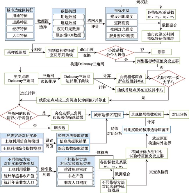
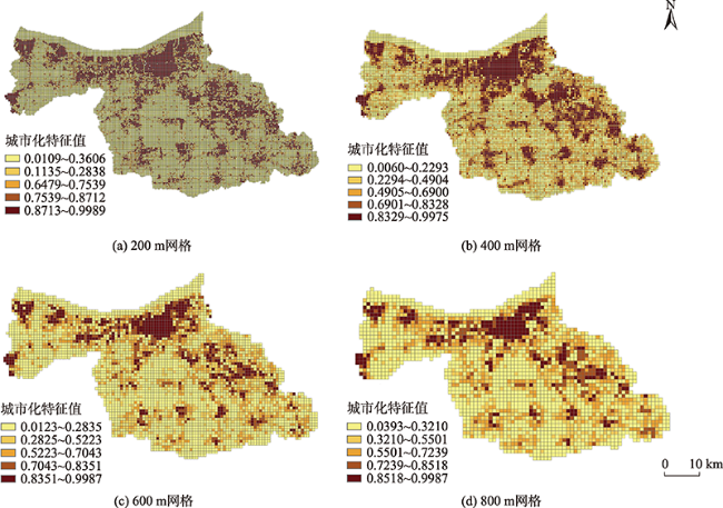
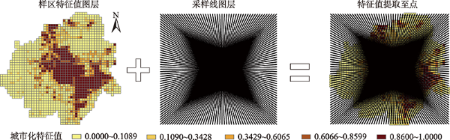
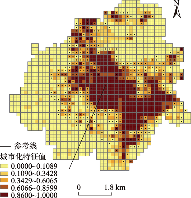
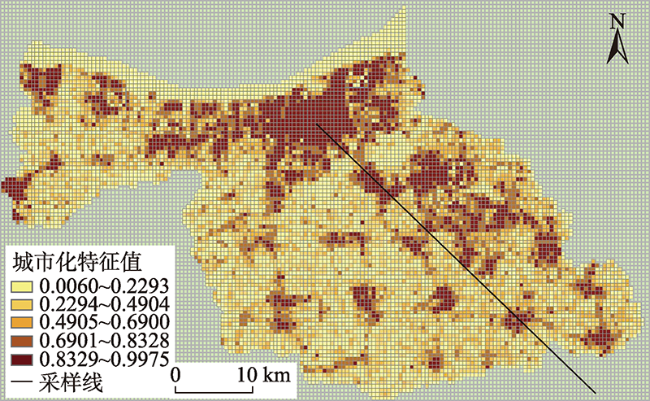
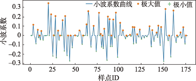
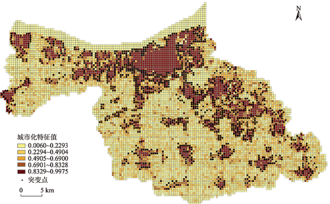
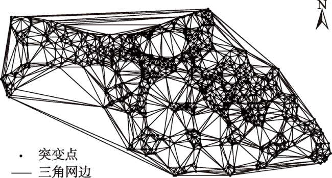
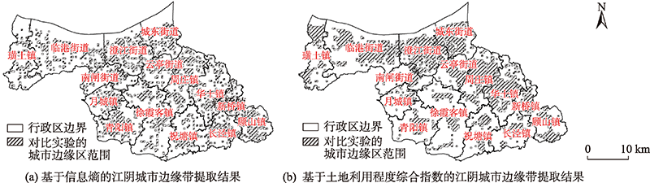
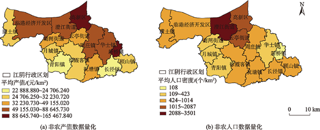
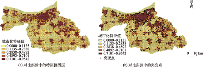
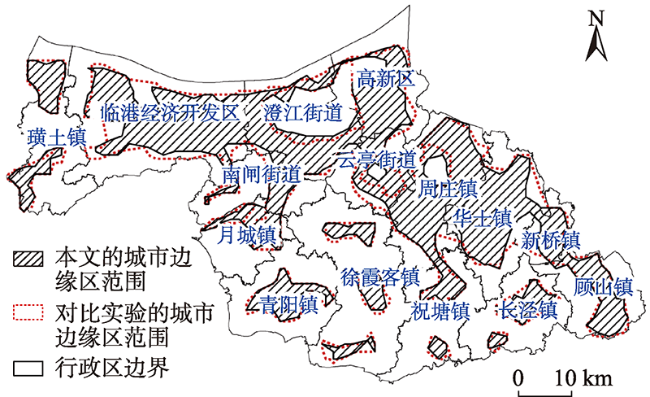
As a transition zone between the city and the countryside, the urban fringe area is not only a geographical space affected by both of the regions, but also an area shrouded in conflicts of interest. The rapid development of urbanization witnesses tremendous changes the urban spatial structure is undergoing. Therefore, studying the spatial scope of the urban fringe area is conducive to the assessment of the current situation of urban development, and is further significant for policy formulation, population management, and resource allocation in the urban fringe area. Thanks to the development of remote sensing and geographic information technology, the types, quality, and accuracy of geospatial data that are applied to depict the characteristics of the urban fringe area have been significantly enhanced. Considering this, this paper takes the spatial mutation characteristics of the urban fringe area as a starting point, and a method for mutation point groups detection, combining multi-indices fusion and wavelet transform, is adopted to distinguish the spatial extent of urban fringe area based on the optimal results by grid-scale evaluation. And then we use the Delaunay triangulation automatic edge length threshold to extract the boundary of the mutation point groups and to obtain the spatial range of the urban fringe area. Empirical analysis is conducted taking Jiangyin City as the research area. The main experimental steps are as follow: firstly, several basic data are selected, containing land use data, road data, night light data, and service-oriented POI data according to the analysis of the characteristics of the urban fringe area. These multi-source data are then standardized based on grids and entropy weighting method for weight determination. In this way, the eigenvalues of the discriminant index of the urban fringe area are calculated. Secondly, based on the spatial mutation characteristics, the wavelet transform is employed to extract the mutation point groups on the eigenvalue sequence, which can effectively improve the discrimination accuracy of the mutation point group. It is suitable for the non-closed circular urban fringe area and for avoiding the influence of human subjective factors. Then, the algorithm based on the Delaunay triangulation automatic edge length threshold is utilized to extract the boundary of the mutation point groups and to obtain the spatial range of the urban fringe area, which can provide a reference for optimizing the urban spatial layout. Finally, the extraction results in this paper are compared with those obtained by the classical methods, like the information entropy model and the comprehensive index model of land use degree. It is apparent to see that the results from classical methods are more chaotic and scattered, while the results in this paper are more complete and objective. Comparing the extraction results of this paper with the extraction results of different index methods employing land use data and administrative division statistical yearbook data to construct urban fringe identification indicators for mutation detection, this study discovers the overlap between them is 88.03%, which testifies the factualness of this method. In terms of the analysis of local details, the results of this paper are more in line with the actual situation. To verify the effectiveness of the method proposed in this paper, the landscape pattern indices are adopted to test the range of urban built-up area, urban fringe area and rural hinterland extracted by the method of this paper and the other different index method respectively. Considering the patch class size landscape pattern indices, the areas delineated by two methods are following the spatial characteristics. Meanwhile, the value of data calculated in the urban fringe area identified in this paper is all higher than the counterpart method given the landscape size landscape pattern indices, the patch density, maximum patch index, landscape separation degree, landscape fragmentation index, and Shannon diversity index. The spread and Shannon uniformity, however, are both lower than the comparison method. It can be indicated that the fragmentation and heterogeneity of the landscape in the urban fringe area identified in this paper is higher, the landscape distribution is uneven, and the socio-economic conditions are more complex, thus proving the effectiveness of this method is especially suitable for the extraction of non-closed circular urban fringe area.

DAI Junjie , DONG Jingwen , YANG Shen , SUN Yizhong . Identification Method of Urban Fringe Area based on Spatial Mutation Characteristics[J]. Journal of Geo-information Science, 2021 , 23(8) : 1401 -1421 . DOI: 10.12082/dqxxkx.2021.200502
表1 不同尺度下的半方差函数参数Tab. 1 Semivariance function parameters under different scales |
| 尺度/m×m | RSS/× | |||||
|---|---|---|---|---|---|---|
| 200×200 | 0.0077 | 0.0626 | 0.1230 | 2910 | 0.5860 | 8.0230 |
| 400×400 | 0.0072 | 0.0520 | 0.1380 | 3270 | 0.6470 | 5.2260 |
| 600×600 | 0.0053 | 0.0423 | 0.1260 | 5310 | 0.6360 | 6.2590 |
| 800×800 | 0.0057 | 0.0400 | 0.1430 | 4680 | 0.6240 | 7.7770 |
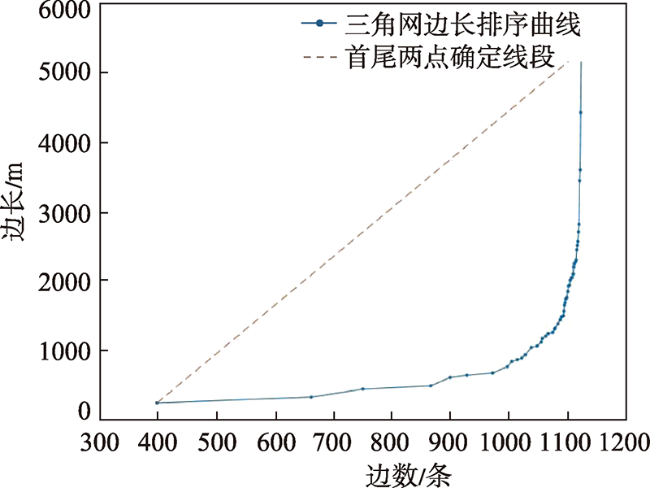
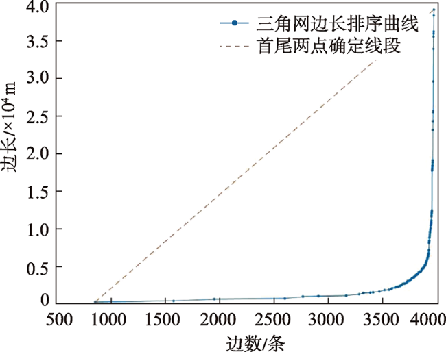
图9 Delaunay三角网边长排序曲线Fig. 9 Curve of lengths of triangle sides resulted from Delaunay triangulation |
表2 土地利用分级指数Tab. 2 Land use classification index |
| 未利用土地级 | 林、草、水用地级 | 农业用地级 | 城镇聚落用地级 | |
|---|---|---|---|---|
| 分级指数 | 1 | 3 | 3 | 4 |
表3 江阴市2017年部分统计年鉴数据Tab. 3 Part statistical yearbook data of Jiangyin City in 2017 |
| 区域名称 | 第二产业产值/万元 | 第三产业产值/万元 | 非农人口/个 |
|---|---|---|---|
| 澄江街道 | 154.750 | 336.600 | 258 039 |
| 南闸街道 | 27.050 | 44.080 | 5456 |
| 高新区 | 378.340 | 199.470 | 72 876 |
| 临港经济开发区 | 417.450 | 295.340 | 81 538 |
| 月城镇 | 31.730 | 27.370 | 6305 |
| 青阳镇 | 32.760 | 33.420 | 8578 |
| 徐霞客镇 | 77.550 | 42.610 | 29 598 |
| 云亭街道 | 50.920 | 51.480 | 28193 |
| 周庄镇 | 240.930 | 100.630 | 46 749 |
| 祝塘镇 | 60.610 | 31.340 | 18 236 |
| 华士镇 | 206.140 | 107.580 | 22 819 |
| 长泾镇 | 29.720 | 32.250 | 20 778 |
| 新桥镇 | 102.020 | 83.090 | 1538 |
| 顾山镇 | 38.960 | 39.930 | 19 091 |
表4 景观格局指数Tab. 4 Landscape pattern index |
| 景观格局指数 | 缩写 | 生态含义 |
|---|---|---|
| 斑块密度 | PD | PD通常用来反映景观总体斑块的分化程度或破碎化程度,斑块密度高表示单位面积斑块的规模小,景观异质性高 |
| 平均斑块面积 | AREA_MN | AREA_MN是指某一斑块类型的总面积除以该类型的斑块数,通常用来反映某种景观破碎化的程度 |
| 最大斑块指数 | LPI | LPI为斑块类型中最大面积的斑块占整体景观面积的比例。该景观格局指数直接体现了景观的优势类型,直接体现了人类活动对于土地利用和景观生态变化的干扰强度和频率的变化 |
| 景观形状指数 | LSI | LSI通过计算某一斑块形状与相同面积的圆或矩形间的偏离程度来测量该形状的复杂程度,反映景观斑块的变异性。LSI值增大时,斑块不规则情况增加 |
| 平均面积权重分维数 | FRAC_AM | FRAC_AM反映景观边界复杂程度 |
| 景观聚集度指数 | AI | AI基于栅格数据来测量景观或某种类型的聚集程度。值小时,表示景观中不同类型的斑块离散程度大;值大时,表示景观中同类型的斑块相互聚合,结构紧凑 |
| 景观结合度指数 | COHESION | COHESION表示景观区域中的景观空间链接度,景观结合度指数值高时表示景观中空间链接度高 |
| 蔓延度 | CONTAG | CONTAG用来反映景观中不同斑块类型的团聚程度和蔓延趋势,高蔓延值表明景观类型中的某种斑块类型形成良好的连接性;反之则表明景观中存在许多小斑块,是具有多种要素的密集格局,景观的破碎化程度较高 |
| 景观分离度 | DIVISION | DIVISION表示某一景观类型中不同景观斑块分布的分离程度;分离度越大,景观在地域分布上越分散,景观分布越复杂,破碎化程度越高 |
| 景观破碎化指数 | SPLIT | SPLIT表征景观被分割的破碎程度,反映景观空间结构的复杂性,在一定程度上反映了人类对景观的干扰程度,进而反映出人类对自然生态系统的影响,一般来说,破碎度越大,人类对生态系统的影响越大 |
| 香农多样性 | SHDI | SHDI用来反映景观类型的丰富和复杂程度,值越大表明景观中没有优势类型且各景观类型趋于均匀分布 |
| 香农均匀度 | SHEI | SHEI反映景观中各斑块类型在面积上分布的均匀程度,其值越趋于1景观分布越均匀 |
表5 本文方法计算的斑块类型层级景观格局指数Tab. 5 Patch class size landscape pattern index table calculated by the method in this paper |
| 景观 | 区域 | AREA_MN | PD | LSI | FRAC_AM | AI | COHESION | DIVISION |
|---|---|---|---|---|---|---|---|---|
| 耕地 | 中心城区 | 23.1111 | 0.1362 | 2.7500 | 1.0117 | 22.2222 | 23.2475 | 0.9998 |
| 边缘区 | 82.2472 | 0.3398 | 18.4918 | 1.0904 | 39.6834 | 72.6685 | 0.9982 | |
| 乡村腹地 | 1242.0000 | 0.0486 | 18.9464 | 1.2388 | 67.0384 | 98.2999 | 0.8350 | |
| 林地 | 边缘区 | 57.6000 | 0.0382 | 5.0000 | 1.0552 | 46.4567 | 63.1566 | 0.9999 |
| 乡村腹地 | 150.2222 | 0.0219 | 5.0769 | 1.0626 | 66.0256 | 77.3700 | 0.9998 | |
| 草地 | 中心城区 | 20.8000 | 0.1513 | 2.8750 | 1.0065 | 16.6667 | 16.1449 | 0.9999 |
| 边缘区 | 21.8537 | 0.0783 | 6.6667 | 1.0232 | 12.3711 | 28.5565 | 1.0000 | |
| 乡村腹地 | 24.5333 | 0.0364 | 5.6429 | 1.0187 | 16.6667 | 25.4607 | 1.0000 | |
| 水域 | 中心城区 | 19.5556 | 0.1362 | 2.8571 | 1.0034 | 13.3333 | 11.6250 | 0.9999 |
| 边缘区 | 25.9200 | 0.1909 | 10.4231 | 1.0201 | 17.7852 | 28.4724 | 1.0000 | |
| 乡村腹地 | 56.5333 | 0.2004 | 10.7755 | 1.0989 | 57.1173 | 84.9260 | 0.9946 | |
| 建设用地 | 中心城区 | 2005.3333 | 0.0454 | 3.1795 | 1.1004 | 88.0785 | 98.3152 | 0.3988 |
| 边缘区 | 561.0847 | 0.1126 | 16.1319 | 1.1734 | 65.9748 | 95.2245 | 0.9308 | |
| 乡村腹地 | 50.8235 | 0.4750 | 25.9296 | 1.0642 | 26.6473 | 56.5048 | 0.9997 |
表6 对比实验计算的斑块类型层级景观格局指数Tab. 6 Patch class size landscape pattern index table calculated by the method in comparison experiment |
| 景观 | 区域 | AREA_MN | PD | LSI | FRAC_AM | AI | COHESION | DIVISION |
|---|---|---|---|---|---|---|---|---|
| 耕地 | 中心城区 | 27.7895 | 0.2399 | 4.3333 | 1.0161 | 25.9259 | 31.0707 | 0.9996 |
| 边缘区 | 105.2727 | 0.2983 | 19.1594 | 1.1048 | 44.2368 | 79.0000 | 0.9967 | |
| 乡村腹地 | 1391.0303 | 0.0444 | 17.8056 | 1.2467 | 67.7620 | 98.6820 | 0.7853 | |
| 林地 | 中心城区 | 16.0000 | 0.0126 | 1.0000 | 1.0000 | - | 0.0000 | 1.0000 |
| 边缘区 | 82.4000 | 0.0339 | 5.1905 | 1.0545 | 52.4324 | 66.2776 | 0.9999 | |
| 乡村腹地 | 141.0000 | 0.0215 | 4.6667 | 1.0591 | 65.8915 | 76.2608 | 0.9998 | |
| 草地 | 中心城区 | 20.0000 | 0.1515 | 3.3750 | 1.0056 | 13.6364 | 14.0103 | 0.9999 |
| 边缘区 | 21.4468 | 0.0797 | 6.9375 | 1.0123 | 13.6364 | 19.9432 | 1.0000 | |
| 乡村腹地 | 23.6190 | 0.0282 | 4.4167 | 1.0152 | 18.0000 | 24.1514 | 1.0000 | |
| 水域 | 中心城区 | 23.1111 | 0.1136 | 2.8750 | 1.0201 | 16.6667 | 25.0755 | 0.9999 |
| 边缘区 | 28.0727 | 0.1865 | 11.1786 | 1.0298 | 20.3911 | 37.3779 | 0.9999 | |
| 乡村腹地 | 58.7020 | 0.2030 | 10.1250 | 1.1001 | 58.6792 | 85.5433 | 0.9937 | |
| 建设用地 | 中心城区 | 2309.3333 | 0.0379 | 3.3810 | 1.0912 | 87.8641 | 97.3064 | 0.6050 |
| 边缘区 | 482.2222 | 0.1221 | 16.8617 | 1.1728 | 64.8846 | 94.7853 | 0.9480 | |
| 乡村腹地 | 45.1337 | 0.5027 | 24.6000 | 1.0576 | 24.9878 | 53.3212 | 0.9997 |
表7 景观层级景观格局指数Tab. 7 Landscape size landscape pattern index table |
| 景观指数 | 本文方法 | 不同指标方法 | |||||
|---|---|---|---|---|---|---|---|
| 建成区 | 边缘区 | 乡村腹地 | 建成区 | 边缘区 | 乡村腹地 | ||
| PD | 0.4691 | 0.7598 | 0.7823 | 0.5556 | 0.7204 | 0.7997 | |
| LPI | 76.7554 | 20.3421 | 39.1059 | 59.5960 | 17.7651 | 45.0538 | |
| LSI | 3.3659 | 16.4304 | 19.6181 | 3.7778 | 16.9795 | 18.5328 | |
| FRAC_AM | 1.0921 | 1.1375 | 1.1730 | 1.0816 | 1.1379 | 1.1791 | |
| AI | 81.7670 | 54.8965 | 55.6802 | 79.4382 | 54.8470 | 56.5867 | |
| COHESION | 95.1307 | 90.4746 | 95.2351 | 92.7071 | 90.1185 | 95.9542 | |
| CONTAG | 72.2574 | 40.8016 | 40.8820 | 70.1049 | 43.3433 | 42.5859 | |
| DIVISION | 0.3985 | 0.9446 | 0.8291 | 0.6044 | 0.9289 | 0.7785 | |
| SPLIT | 1.6624 | 18.0450 | 5.8515 | 2.5279 | 14.0619 | 4.5153 | |
| SHDI | 0.3180 | 0.8430 | 0.5750 | 0.4550 | 0.8360 | 0.5990 | |
| SHEI | 0.2884 | 0.5894 | 0.6518 | 0.3179 | 0.6211 | 0.6383 | |
| [1] |
|
| [2] |
|
| [3] |
|
| [4] |
|
| [5] |
张晓军. 国外城市边缘区研究发展的回顾及启示[J]. 国际城市规划, 2005, 20(4):72-75.
[
|
| [6] |
顾朝林, 陈田, 丁金宏. 中国大城市边缘区特性研究[J]. 地理学报, 1993, 60(4):317-328.
[
|
| [7] |
顾朝林, 甄峰, 张京祥. 集聚与扩散:城市空间结构新论[M]. 南京: 东南大学出版社, 2000.
[
|
| [8] |
赵自胜, 陈金. 城乡结合部土地利用研究──以开封市为例[J]. 河南大学学报(自然科学版), 1996(01):67-70.
[
|
| [9] |
王树良, 李爽, 刘建华, 等. 试论城乡结合部的土地用途管制[J]. 测绘信息与工程, 2000(4):15-19.
[
|
| [10] |
李世峰, 白人朴. 基于模糊综合评价的大城市边缘区地域特征属性的界定[J]. 中国农业大学学报, 2005, 10(3):99-104.
[
|
| [11] |
刘星南, 吴志峰, 骆仁波, 等. 基于多源数据和深度学习的城市边缘区判定[J]. 地理研究, 2020, 39(2):243-256.
[
|
| [12] |
蔡栋, 李满春, 陈振杰, 等. 基于信息熵的城市边缘区的界定方法研究——以南京市为例[J]. 测绘科学, 2010, 35(3):106-109.
[
|
| [13] |
琚青青, 尹菡怿, 李微, 等. 海口市城市边缘区空间范围的识别研究[J]. 海南大学学报:自然科学版, 2019(2):180-185.
[
|
| [14] |
林坚, 汤晓旭, 黄斐玫, 等. 城乡结合部的地域识别与土地利用研究——以北京中心城地区为例[J]. 城市规划, 2007(8):36-44.
[
|
| [15] |
王秀兰, 李雪瑞, 冯仲科. 基于TM影像的北京城市边缘带范围界定方法研究[J]. 遥感信息, 2010(4):100-104,134.
[
|
| [16] |
马晶, 李全, 应玮. 基于小波变换的武汉市城乡边缘带识别[J]. 武汉大学学报·信息科学版, 2016, 41(2):235-241.
[
|
| [17] |
熊念. 武汉市城市边缘区识别及动态分析[D]. 武汉:武汉大学, 2018.
[
|
| [18] |
张宁, 方琳娜, 周杰, 等. 北京城市边缘区空间扩展特征及驱动机制[J]. 地理研究, 2010(3):91-100.
[
|
| [19] |
赵华甫, 朱玉环, 吴克宁, 等. 基于动态指标的城乡交错带边界界定方法研究[J]. 中国土地科学, 2012, 26(9):60-65.
[
|
| [20] |
周小驰, 刘咏梅, 杨海娟. 西安市城市边缘区空间识别与边界划分[J]. 地球信息科学学报, 2017, 19(10):1327-1335.
[
|
| [21] |
刘戎. 基于土地利用的城市边缘区界定及其空间扩展分析研究[D]. 西安:西北大学, 2017.
[
|
| [22] |
曹广忠, 缪杨兵, 刘涛. 基于产业活动的城市边缘区空间划分方法——以北京主城区为例[J]. 地理研究, 2009, 28(3):771-780.
[
|
| [23] |
雷志成. 基于POI的城市边缘区识别与空间分析[D]. 广州:广州大学, 2019.
[
|
| [24] |
边振兴, 王晓良. 基于RS、GIS的沈阳城市边缘区界定研究[A].中国自然资源学会土地资源研究专业委员会、中国地理学会农业地理与乡村发展专业委员会、青海民族大学公共管理学院.2013全国土地资源开发利用与生态文明建设学术研讨会论文集[C]. 中国自然资源学会土地资源研究专业委员会、中国地理学会农业地理与乡村发展专业委员会、青海民族大学公共管理学院:青海民族大学公共管理学院, 2013: 7.
[
|
| [25] |
吴康敏, 张虹鸥, 王洋 等. 广州市多类型商业中心识别与空间模式[J]. 地理科学进展, 2016, 35(8):963-974.
[
|
| [26] |
|
| [27] |
崔功豪, 武进. 中国城市边缘区空间结构特征及其发展——以南京等城市为例[J]. 地理学报, 1990, 45(4):399-411.
[
|
| [28] |
邢厚道, 杨山. 城市边缘区演化及其特征[J]. 安徽农业科学, 2006(20):5382-5384.
[
|
| [29] |
王海鹰, 张新长, 康停军, 等. 基于多准则判断的城市边缘区界定及其特征[J]. 自然资源学报, 2011, 26(4):703-714.
[
|
| [30] |
|
| [31] |
靳鑫洋, 王素元, 聂建亮, 等. 一种基于Delaunay三角网边长阈值与激光点云的建筑立面结构提取方法[J]. 地理与地理信息科学, 2019, 35(5):80-84.
[
|
| [32] |
|
| [33] |
|
| [34] |
李春光, 汪善勤, 吕叙杰 等. 城市边缘区划分方法初探[J]. 华中师范大学学报(自科版), 2012, 46(2):239-244.
[
|
| [35] |
孙洪泉. 地质统计学及其应用[M]. 徐州: 中国矿业大学出版社, 1990.
[
|
| [36] |
李灿, 张凤荣, 朱泰峰 等. 大城市边缘区景观破碎化空间异质性——以北京市顺义区为例[J]. 生态学报, 2013, 33(17):5363-5374.
[
|
| [37] |
程欢. 西安市文化产业空间异质性多尺度研究[D]. 西安:陕西师范大学, 2016.
[
|
| [38] |
李亮, 吴瑞明. 消除评价指标相关性的权值计算方法[J]. 系统管理学报, 2009, 18(2):221-225.
[
|
| [39] |
徐祥发, 肖人彬. 评价指标相关性的消除方法研究[J]. 系统工程理论与实践, 2002(11):1-5.
[
|
| [40] |
张大陆, 杨哲, 姚进. 分布式电子商务中服务评价指标相关性消除方法[J]. 同济大学学报(自然科学版), 2006(3):401-404.
[
|
| [41] |
|
| [42] |
|
| [43] |
刘纪远. 中国资源环境遥感宏观调查与动态研究[M]. 北京: 中国科学技术出版社, 1996.
[
|
| [44] |
刘崇刚, 孙伟, 曹玉红, 等. 大都市区城乡空间边界演化识别方法研究——以南京市为例[J]. 长江流域资源与环境, 2018, 27(10):65-72.
[
|
| [45] |
江阴市统计局. 江阴统计年鉴.2017[M]. 北京: 中国统计出版社, 2017.
[Jiangyin Bureau of Statistics. Jiangyin statistical yearbook 2017[M]. Beijing: China Statistics Press, 2017. ]
|
| [46] |
李广东, 戚伟. 中国建设用地扩张对景观格局演化的影响[J]. 地理学报, 2019, 74(12):2572-2591.
[
|
| [47] |
|
| [48] |
|
| [49] |
|
/
| 〈 |
|
〉 |
