
Journal of Geo-information Science >
Bayesian Geostatistical Modelling for Precipitation Data with Nested Anisotropy Measured at Sparse Reference Stations
Received date: 2021-11-15
Revised date: 2022-02-18
Online published: 2022-10-25
Supported by
National Natural Science Foundation of China(42001265)
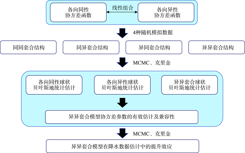
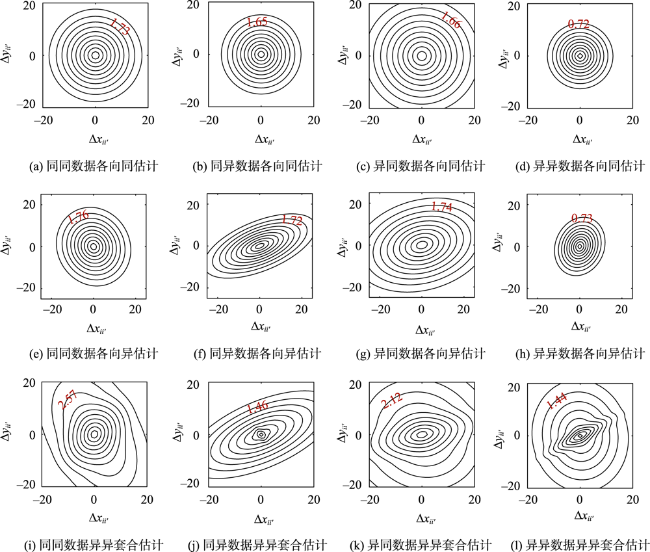
Spatially continuous precipitation data are important data input in hydrological simulation in a watershed, hydrological modeling of land surface, eco-environmental sensitivity evaluation, comprehensive investigation and zoning of geographical environment, and so on. These data are often interpolated from the discrete observations of monitoring points. However, due to the operations and interactions of the underlying physical processes on different scales, the spatial variations of precipitation are generally viewed as a result of the superposition of different geographical processes on multiple scales and directions. The multi-scale, multi-direction natures of geographical processes determine the weights between spatial points, which have an important impact on spatial interpolation. Therefore, it is necessary to establish a multi-scale and multi-direction spatial model to better reflect the dynamic process for regional precipitation estimation and spatial analysis, especially in sparse monitoring areas. Bayesian geostatistical models have the ability of multi-scale and multi-direction modeling and provide a scalable statistical inference framework by integrating observations (external implementation with errors), unknown variables, prior information, and complex dynamical models (real processes). In view of the superposition phenomena of precipitation on scales and directions, this study explored the possibility of decomposition estimates for the sparse data with nested anisotropy based on Bayesian and geostatistical methods to accurately determine the contribution of each independent component. We also further demonstrated the application potential of this model in precipitation interpolation. The results showed that, firstly, the nested anisotropy and multi-scale properties hidden in the sparse data could be well estimated by the Bayesian and geostatistical methods applied in the four random simulations with nested structures using a Fourier integration method. The more complex the model was, the more difficult the estimation was and the stronger the uncertainty was, and the convergence and estimation accuracy could be improved by introducing some prior information. The interpolation accuracy of the heterogeneous models was better than that of the models with simple isotropy or anisotropy. And also the more complex the covariance structure of the data was, the more obvious the improvement effect was. Secondly, complex structures had the ability of downward compatibility with simple structures, but simple structures did not have the ability of upward compatibility with complex structures. Finally, based on the interpolation results, the nested model played an obvious role in improving the accuracy of regional precipitation interpolation, which was about 10% higher than the estimation accuracy of the two basic models. Compared with the two basic structures, the method in this study not only identified two kinds of superposition information but also obtained the contributions of the two components, with a contribution ratio close to 1:1.
GAO Xin , YUAN Shengyuan , LI Jingzhong , ZHAO Huibing , XU Shuna . Bayesian Geostatistical Modelling for Precipitation Data with Nested Anisotropy Measured at Sparse Reference Stations[J]. Journal of Geo-information Science, 2022 , 24(8) : 1445 -1458 . DOI: 10.12082/dqxxkx.2022.210729
表1 4种球状套合协方差矩阵的计算公式和参数空间Tab. 1 The formulas and parameter spaces of covariance matrices for the four spherical models with nested structures |
| 结构 | 公式 | 参数空间 | 参数说明 | 公式编号 |
|---|---|---|---|---|
| 同同套合 | {μ,τ2, , ,a1,a2}, a1 ≤ a2 | μ:均值;τ2:块金值; :结构1方差; :结构2方差;a1:结构1变程;a2:结构2变程 | (6) | |
| 同异套合 | {μ,τ2, , ,a1,a2,min,a2,max,β2}, a1 ≤ a2,min≤a2,max | μ:均值;τ2:块金值; :结构1方差; :结构2方差;a1:结构1变程;a2,min,:结构2变程短半径;a2,max:结构2变程长半径;β2:结构2倾角 | (7) | |
| 异同套合 | {μ,τ2, , ,a1,min,a1,max,a2,β1}, a1,min≤ a1,max≤ a2 | μ:均值;τ2:块金值; :结构1方差; :结构2方差;a1,min:结构1变程短半径,a1,max:结构1变程长半径;a2:结构2变程;β1:结构1倾角 | (8) | |
| 异异套合 | {μ,τ2, , ,a1,min,a1,max,a2,min, a2,max,β1,β2}, a1,min≤ a1,max≤ a2,min≤ a2,max | μ:均值;τ2:块金值; :结构1方差; :结构2方差;a1,min:结构1变程短半径,a1,max:结构1变程长半径;结构2变程短半径;a2,max:结构2变程长半径; β1:结构1倾角;β2:结构2倾角 | (9) |
表2 4种套合模拟数据的协方差参数值Tab. 2 The values of covariance parameters for the four nested simulation data |
| 同同套合 | 取值 | 同异套合 | 取值 | 异同套合 | 取值 | 异异套合 | 取值 |
|---|---|---|---|---|---|---|---|
| μ | 0 | μ | 0 | μ | 0 | μ | 0 |
| 5 | 3 | 3 | 5 | ||||
| 5 | 7 | 7 | 5 | ||||
| a1 | 15 | a1 | 15 | a1,min | 15 | a1,min | 8 |
| a2 | 40 | a2,min | 20 | a1,max | 30 | a1,max | 16 |
| a2,max | 40 | a2 | 40 | a2,min | 20 | ||
| β2 | π/6 | β1 | π/6 | a2,max | 40 | ||
| β1 | π/6 | ||||||
| β2 | π/2 |
表3 各向同性模型用于4种套合数据的分位数估计(2.5%, 50%, 97.5%)Tab. 3 The quantile estimates (2.5%, 50%, 97.5%) for the four simulations using an isotropic model |
| 参数 | 同同套合 | 同异套合 | 异同套合 | 异异套合 | |||||||||||
|---|---|---|---|---|---|---|---|---|---|---|---|---|---|---|---|
| 2.5% | 50% | 97.5% | 2.5% | 50% | 97.5% | 2.5% | 50% | 97.5% | 2.5% | 50% | 97.5% | ||||
| μ | 0.02 | 0.36 | 0.73 | -0.14 | 0.18 | 0.49 | -0.47 | -0.07 | 0.39 | -0.01 | 0.26 | 0.53 | |||
| σ2 | 8.39 | 9.49 | 11.05 | 7.82 | 9.07 | 10.50 | 8.03 | 9.15 | 9.97 | 7.02 | 7.87 | 8.86 | |||
| a | 21.45 | 23.75 | 27.17 | 17.24 | 20.39 | 23.69 | 25.39 | 29.28 | 37.21 | 15.30 | 16.77 | 18.73 | |||
| RMSE | 2.3262 | 3.6353 | 2.1857 | 2.6992 | |||||||||||
表4 各向异性模型用于4种套合数据的分位数估计(2.5%, 50%, 97.5%)Tab. 4 The quantile estimates (2.5%, 50%, 97.5%) for the four simulations using an anisotropic model |
| 参数 | 同同套合 | 同异套合 | 异同套合 | 异异套合 | |||||||||||
|---|---|---|---|---|---|---|---|---|---|---|---|---|---|---|---|
| 2.5% | 50% | 97.5% | 2.5% | 50% | 97.5% | 2.5% | 50% | 97.5% | 2.5% | 50% | 97.5% | ||||
| μ | 0.02 | 0.38 | 0.73 | -0.06 | 0.30 | 0.65 | -0.64 | -0.13 | 0.34 | -0.02 | 0.25 | 0.55 | |||
| σ2 | 8.54 | 9.70 | 11.09 | 8.27 | 9.47 | 11.03 | 8.36 | 9.59 | 9.92 | 7.14 | 8.02 | 9.33 | |||
| amin | 20.25 | 23.19 | 26.90 | 12.07 | 15.92 | 18.01 | 17.99 | 28.89 | 31.21 | 13.23 | 15.59 | 18.64 | |||
| amax | 22.77 | 25.81 | 29.85 | 30.89 | 38.15 | 44.00 | 38.99 | 44.18 | 52.66 | 16.07 | 19.23 | 25.11 | |||
| β | 0.05 | 2.06 | 3.10 | 0.27 | 0.39 | 0.57 | 0.06 | 0.27 | 3.13 | 0.21 | 1.18 | 2.90 | |||
| RMSE | 2.3343 | 3.6691 | 2.2126 | 2.6905 | |||||||||||
表5 异异套合模型用于4种套合数据的分位数估计(2.5%, 50%, 97.5%)Tab. 5 The quantile estimates (2.5%, 50%, 97.5%) for the four simulations using a nested model with anisotropy and anisotropy |
| 参数 | 同同套合 | 同异套合 | 异同套合 | 异异套合 | |||||||||||
|---|---|---|---|---|---|---|---|---|---|---|---|---|---|---|---|
| 2.5% | 50% | 97.5% | 2.5% | 50% | 97.5% | 2.5% | 50% | 97.5% | 2.5% | 50% | 97.5% | ||||
| μ | -0.04 | 0.33 | 0.73 | -0.04 | 0.32 | 0.65 | -0.50 | -0.07 | 0.33 | -0.16 | 0.16 | 0.50 | |||
| 0.03 | 4.08 | 8.23 | 0.73 | 1.27 | 1.95 | 1.69 | 2.75 | 3.72 | 1.62 | 2.67 | 3.92 | ||||
| 1.30 | 5.33 | 9.93 | 5.50 | 6.77 | 8.17 | 4.17 | 5.02 | 6.51 | 3.65 | 5.27 | 6.96 | ||||
| a1,min | 1.33 | 12.84 | 21.93 | 0.23 | 2.24 | 4.57 | 4.78 | 9.66 | 11.14 | 2.03 | 3.91 | 6.58 | |||
| a1,max | 2.60 | 20.87 | 25.38 | 2.11 | 5.90 | 13.90 | 25.20 | 30.13 | 32.53 | 13.75 | 21.54 | 29.21 | |||
| a2,min | 21.19 | 26.69 | 44.99 | 15.20 | 17.58 | 19.84 | 35.13 | 38.57 | 43.62 | 22.98 | 26.79 | 30.75 | |||
| a2,max | 23.29 | 48.00 | 62.23 | 36.14 | 42.16 | 48.55 | 39.85 | 43.76 | 51.10 | 27.02 | 31.50 | 48.21 | |||
| β1 | 0.03 | 0.80 | 3.11 | 0.05 | 2.26 | 3.11 | 0.10 | 0.24 | 3.13 | 0.27 | 0.49 | 0.61 | |||
| β2 | 0.16 | 2.07 | 3.01 | 0.30 | 0.41 | 0.52 | 0.01 | 2.60 | 2.74 | 0.26 | 1.73 | 2.82 | |||
| RMSE | 2.2998 | 3.5819 | 2.1831 | 2.6225 | |||||||||||
表6 3种模型应用于降水数据中的分位数估计(2.5%, 50%, 97.5%)Tab. 6 The quantile estimates(2.5%, 50%, 97.5%) for precipitation data using the three models including an isotropic, an anisotropic and a nested model with anisotropy and anisotropy |
| 参数 | 各向同性模型 | 各向异性模型 | 异异套合模型 | ||||||||
|---|---|---|---|---|---|---|---|---|---|---|---|
| 2.5% | 50% | 97.5% | 2.5% | 50% | 97.5% | 2.5% | 50% | 97.5% | |||
| μ/mm | 6.12 | 6.16 | 6.18 | 6.12 | 6.14 | 6.16 | 6.13 | 6.15 | 6.19 | ||
| τ2/mm2 | 1.45E-03 | 2.31E-03 | 3.04E-03 | 3.06E-05 | 7.06E-04 | 1.61E-03 | 2.24E-05 | 5.07E-04 | 1.53E-03 | ||
| σ2/mm2 | 1.48E-02 | 1.62E-02 | 1.68E-02 | 1.34E-02 | 1.52E-02 | 1.68E-02 | 5.19E-03 | 8.34E-03 | 9.23E-03 | ||
| - | - | - | - | - | - | 5.92E-03 | 8.60E-03 | 1.51E-02 | |||
| a/km | amin | a1,min | 181.70 | 253.30 | 270.96 | 86.37 | 97.74 | 119.64 | 67.28 | 83.08 | 86.29 |
| a1,max | - | - | - | - | - | - | 176.06 | 210.49 | 250.03 | ||
| amax | a2,min | - | - | - | 178.67 | 237.96 | 272.50 | 196.82 | 237.39 | 292.93 | |
| a2,max | - | - | - | - | - | - | 267.80 | 290.50 | 304.16 | ||
| β | β1 | - | - | - | 1.15 | 1.39 | 1.60 | 1.33 | 1.48 | 1.54 | |
| β2 | - | - | - | - | - | - | 0.06 | 0.43 | 3.07 | ||
| RMSE/mm | 22.14 | 22.21 | 20.07 | ||||||||
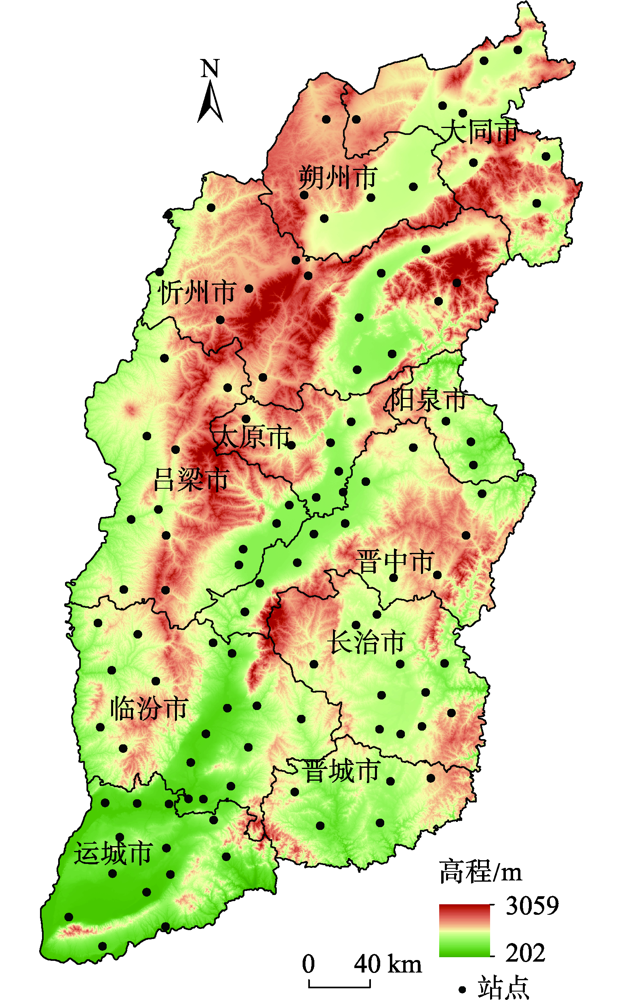
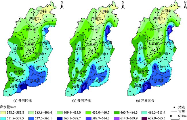
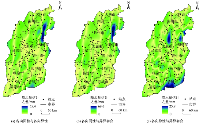
图6 各向同性、各向异性和异异套合模型的插值结果Fig. 6 The interpolation results using an isotropic, an anisotropic and a nested model with anisotropy and anisotropy for the precipitation data measured in Shanxi province |
| [1] |
郑度, 欧阳, 周成虎. 对自然地理区划方法的认识与思考[J]. 地理学报, 2008, 63(6):563-573.
[
|
| [2] |
陈广宇, 韦志刚, 董文杰, 等. 中国西部陆面过程次网格地形参数化的改进对区域气温和降水模拟的影响研究[J]. 大气科学, 2019, 43(4):846-860.
[
|
| [3] |
范泽孟. 中国生态过渡带分布的空间识别及情景模拟[J]. 地理学报, 2021, 76(3):626-644.
[
|
| [4] |
|
| [5] |
|
| [6] |
|
| [7] |
|
| [8] |
|
| [9] |
|
| [10] |
|
| [11] |
|
| [12] |
|
| [13] |
|
| [14] |
|
| [15] |
|
| [16] |
|
| [17] |
|
| [18] |
|
| [19] |
|
| [20] |
|
| [21] |
|
| [22] |
|
| [23] |
|
| [24] |
|
| [25] |
|
| [26] |
|
| [27] |
|
| [28] |
|
| [29] |
|
| [30] |
高歆. 基于线性GSI二维半变异函数各向异性结构建模及估计研究——以DEM数据为例[J]. 地理研究, 2020, 39(11):2607-2625.
[
|
| [31] |
王劲峰, 徐成东. 地理探测器:原理与展望[J]. 地理学报, 2017, 72(1):116-134.
[
|
| [32] |
葛咏, 刘梦晓, 胡姗, 等. 时空统计学在贫困研究中的应用及展望[J]. 地球信息科学学报, 2021, 23(1):58-74.
[
|
| [33] |
|
| [34] |
|
| [35] |
中国地面气候标准值年值数据集(1981-2010)[DB/OL]. 国家气象科学数据中心
[The annual normalized dataset of surface climate in China 1981-2010)[DB/OL]. China Meteorological Data Service Center ]
|
| [36] |
|
| [37] |
|
/
| 〈 |
|
〉 |