
Journal of Geo-information Science >
Chlorophyll-a Concentration Inversion Model: Stacked Auto-encoder Particle Swarm Optimization BP Neural Network
Received date: 2023-03-23
Revised date: 2023-06-05
Online published: 2023-09-05
Supported by
High Resolution Earth Observation System is a Major National Science and Technology Project(67-Y50G04-9001-22/23)
High Resolution Earth Observation System is a Major National Science and Technology Project(67-Y50G05-9001-22/23)
Science and Technology Research Project of Education Department of Hebei Province(CXY2023011)
Science and Technology Research Project of Education Department of Hebei Province(QN2022076)
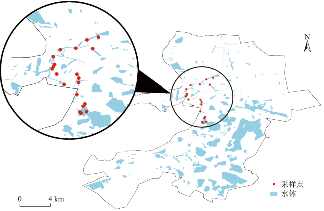
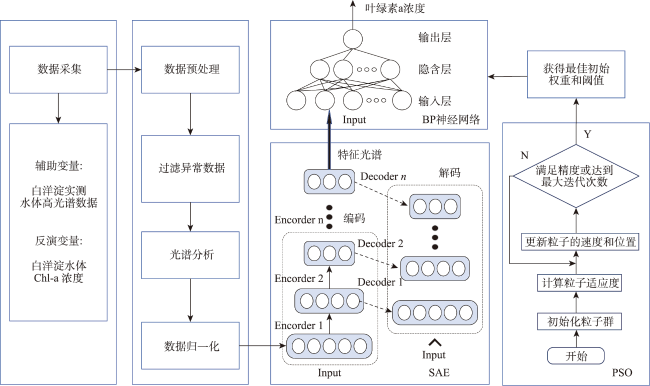
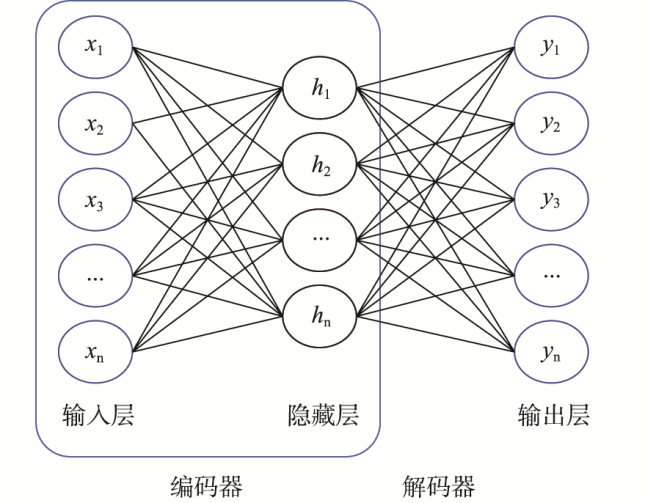
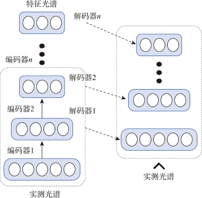
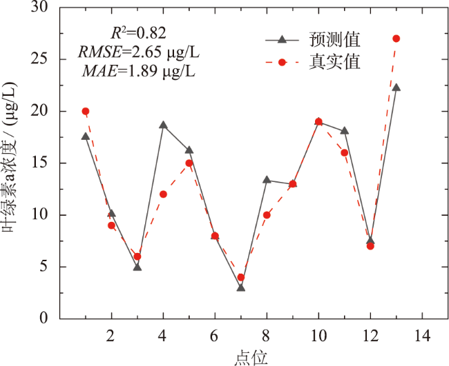
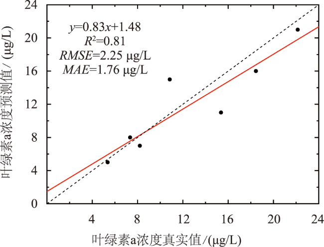
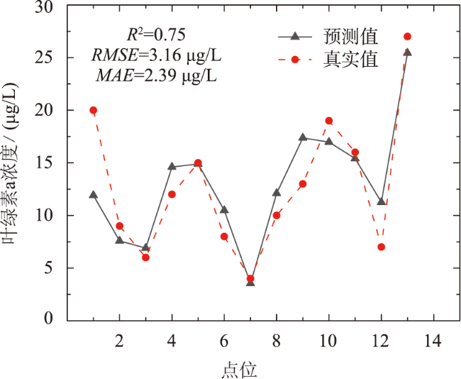
The concentration of Chlorophyll-a(Chl-a) has been the main indicator of eutrophication of inland waters and one of the important factors affecting the spectral characteristics of the reflectance of water. Monitoring the concentration of Chl-a in inland water bodies can provide valuable information for managing and mitigating the effects of eutrophication. In this study, hyperspectral data and water samples were collected from Baiyangdian Lake and villages in Baotou County, and water quality parameters such as Chl-a were determined in the laboratory, which were applied to Chl-a hyperspectral remote sensing inversion in Baiyangdian region. The stacked auto-encoder particle swarm optimization BP neural network model, the BP neural network model of hyperspectral data without dimensionality reduction, the BP neural network model of dimensionality reduction based on principal component analysis, and the BP neural network model of dimensionality reduction based on stepwise regression analysis were respectively established. To solve the problems of insufficient feature extraction ability of linear dimension reduction method and low learning efficiency and poor generalization ability of Chl-a hyperspectral remote sensing inversion model constructed by neural network, an inversion model of Chl-a concentration was proposed based on stacked auto-encoder particle swarm optimization BP neural network. This model used the powerful nonlinear transformation ability of stacked auto-encoder to learn the features of hyperspectral data by minimizing the reconstruction error. It achieved the dimensionality reduction of data while preserving the radiation information of the original spectral data to the greatest extent, and extracted the depth features of the measured water spectrum. The initial weight of BP neural network was taken as the position vector of the particle. Particle swarm optimization algorithm was used to search for the optimal initial weight of the network, reduce the probability of local extreme value, and improve the stability of the model and the accuracy of inversion. Compared to the BP neural network model without dimensionality reduction of hyperspectral data (R2=0.75, RMSE=3.16 μg/L, MAE=2.39 μg/L), the BP neural network model based on principal component analysis for dimensionality reduction (R2=0.79, RMSE=2.85 μg/L, MAE=2.29 μg/L), and the BP neural network model based on stepwise regression analysis for dimensionality reduction (R2=0.80, RMSE=2.79 μg/L, MAE=2.38 μg/L), the stacked auto-encoder particle swarm optimization BP neural network model (R2=0.82, RMSE=2.65 μg/L, MAE=1.89 μg/L) had higher accuracy in hyperspectral remote sensing inversion of Chl-a in inland water bodies. This study provides a theoretical basis and technical support for hyperspectral remote sensing inversion of Chl-a in inland Class II water bodies, helps with continuous monitoring of water quality in Baiyangdian Lake, and provides new ideas for future hyperspectral satellite remote sensing image inversion of Chl-a.

HAN Baohui , ZHAO Qichao , CHANG Rong , LI Xiaomeng , YAN Keqin , FU Qiming . Chlorophyll-a Concentration Inversion Model: Stacked Auto-encoder Particle Swarm Optimization BP Neural Network[J]. Journal of Geo-information Science, 2023 , 25(9) : 1882 -1893 . DOI: 10.12082/dqxxkx.2023.230144
表1 水体采样点统计Tab.1 Statistical table of water body sampling points |
| 点位 | 周边村名 | 经度/ E | 纬度/ N | Chl-a(μg/L) |
|---|---|---|---|---|
| 1 | 寨南村 | 115°59′17.9*″ | 38°54′3.0*″ | 16 |
| 2 | 泥李庄村 | 115°58′59.3*″ | 38°54′29.0*″ | 20 |
| 3 | 噶子村 | 115°58′47.7*″ | 38°54′42.2*″ | 21 |
| 4 | 噶子村 | 115°58′50.7*″ | 38°54′47.6*″ | 16 |
| 5 | 噶子村 | 115°58′53.9*″ | 38°54′53.2*″ | 19 |
| 6 | 小张庄村 | 115°58′50.7*″ | 38°55′13.1*″ | 9 |
| 7 | 大张庄村 | 115°59′8.1*″ | 38°55′30.9*″ | 6 |
| 8 | 大张庄村 | 115°59′47.7*″ | 38°55′34.9*″ | 7 |
| 9 | 郭里口村 | 116°0′16.0*″ | 38°55′56.2*″ | 8 |
| 10 | 郭里口村 | 116°0′45.6*″ | 38°56′3.4*″ | 8 |
| 11 | 郭里口村 | 116°0′31.0*″ | 38°55′33.8*″ | 4 |
| 12 | 王家寨村 | 115°59′50.5*″ | 38°54′28.8*″ | 5 |
| 13 | 寨南村 | 115°59′55.2*″ | 38°54′18.8*″ | 13 |
| 14 | 寨南村 | 115°59′54.7*″ | 38°54′7.7*″ | 7 |
| 15 | 寨南村 | 115°59′50.7*″ | 38°53′36.8*″ | 11 |
| 16 | 东淀头村 | 116°0′10.9*″ | 38°53′12.6*″ | 10 |
| 17 | 东淀头村 | 116°0′6.1*″ | 38°53′6.5*″ | 12 |
| 18 | 东淀头村 | 115°59′58.0*″ | 38°52′51.2*″ | 15 |
| 19 | 东淀头村 | 116°0′1.1*″ | 38°52′48.1*″ | 27 |
| 20 | 东淀头村 | 116°0′15.3*″ | 38°52′51.9*″ | 15 |
注:表中用*代替详细的经纬度信息。 |
表2 SAE-PSO-BP网络预测模型参数Tab. 2 Parameters of SAE-PSO-BP network prediction model |
| 参数 | 值 |
|---|---|
| PSO学习因子 | 1.50 |
| PSO学习因子 | 1.50 |
| PSO初始种群数 | 400 |
| PSO最大迭代次数 | 10 |
| PSO初始粒子随机速度 | (-1,1) |
| PSO初始粒子随机位置 | (0,0.1) |
| PSO的惯性因子w | 1.1 |
| PSO-BP训练次数 | 5 000 |
| PSO-BP学习率 | 0.02 |
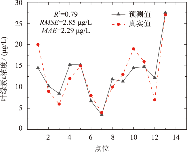
图9 PCA-BP模型反演Chl-a结果Fig. 9 Inversion of Chl-a results by PCA-BP modelnetwork model without reduced dimension |
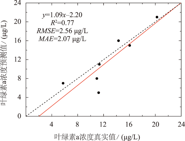
图12 PCA-BP模型反演结果精度Fig. 12 Accuracy of PCA-BP model inversion resultswithout reducing dimension |
表3 4种模型的精度验证统计Tab. 3 Accuracy verification statistics table of the four models |
| 方法模型 | R2 | RMSE/(μg/L) | MAE/(μg/L) | |
|---|---|---|---|---|
| 训练集 | 不降维BP神经网络模型 | 0.75 | 3.16 | 2.39 |
| PCA-BP模型 | 0.79 | 2.85 | 2.29 | |
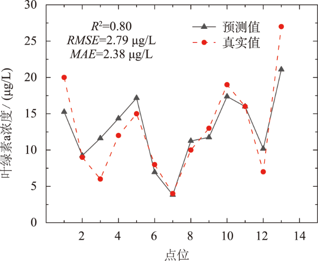
| SR-BP模型 | 0.80 | 2.79 | 2.38 | |
| SAE-PSO-BP模型 | 0.82 | 2.65 | 1.89 | |
| 验证集 | 不降维BP神经网络模型 | 0.73 | 2.75 | 2.56 |
| PCA-BP模型 | 0.77 | 2.56 | 2.07 | |
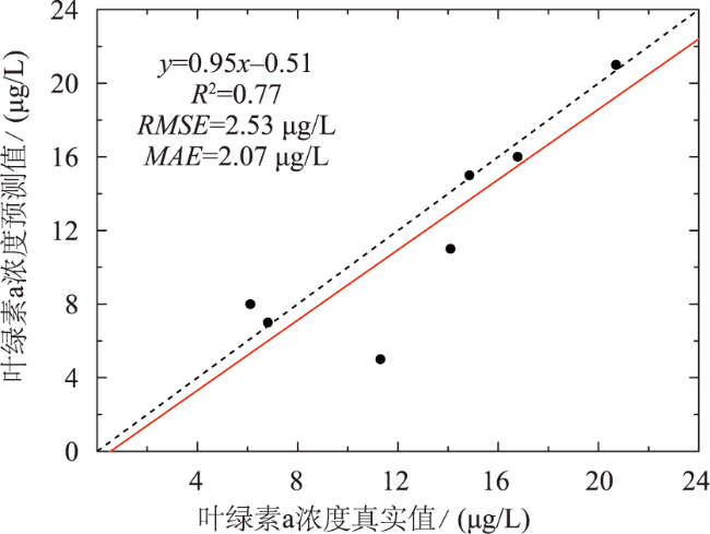
| SR-BP模型 | 0.77 | 2.53 | 2.07 | |
| SAE-PSO-BP模型 | 0.81 | 2.25 | 1.76 |
| [1] |
|
| [2] |
詹志薇, 谭志, 金腊华, 等. 水源型水库的氮形态分布特征与水体富营养化的关系[J]. 安徽农业科学, 2017, 45(10):59-62.
[
|
| [3] |
韩耀全, 黄励, 施军, 等. 常用水体初级生产力测定方法的结果差异分析[J]. 江苏农业科学, 2018, 46(1):201-206.
[
|
| [4] |
金松, 韩震, 李雪娜, 等. 叶绿素浓度和海表温度与黄海绿潮海洋初级生产力关系的研究[J]. 海洋湖沼通报, 2017(2):131-138.
[
|
| [5] |
冯世敏, 刘冬燕, 李东京, 等. 安徽太平湖水库初级生产力时空分布及分析[J]. 湖泊科学, 2016, 28(6):1361-1370.
[
|
| [6] |
郭诗君, 王小军, 韩品磊, 等. 丹江口水库叶绿素a浓度的时空特征及影响因子分析[J]. 湖泊科学, 2021, 33(2):366-376.
[
|
| [7] |
李恺霖, 廖廓, 党皓飞. 内陆与近岸水体的色度学遥感研究进展[J]. 自然资源遥感, 2023, 35(1):15-26.
[
|
| [8] |
朱云芳. 基于GF-1WFV影像和BP神经网络的太湖叶绿素a反演[J]. 环境科学学报, 2017, 37(1):130-137.
[
|
| [9] |
|
| [10] |
|
| [11] |
孙茜童, 付芸, 韩春晓, 等. 基于卷积神经网络的全球海洋叶绿素a浓度反演方法[J]. 光谱学与光谱分析, 2023, 43(2): 608-613.
[
|
| [12] |
|
| [13] |
|
| [14] |
|
| [15] |
曹红业, 龚涛, 袁成忠, 等. 基于RBF模型的太湖北部叶绿素a浓度定量遥感反演[J]. 环境工程学报, 2016, 10(11):6499-6504.
[
|
| [16] |
|
| [17] |
|
| [18] |
杨承恩, 苏玲, 冯伟志, 等. 中红外光谱结合机器学习对不同产地平菇鉴别[J]. 光谱学与光谱分析, 2023, 43(2):577-582.
[
|
| [19] |
张晓东, 李立, 毛罕平, 等. 基于PCA-BP多特征融合的油菜水分胁迫无损检测[J]. 江苏大学学报(自然科学版), 2016, 37(2):174-182.
[
|
| [20] |
潘月, 曹宏鑫, 齐家国, 等. 基于高光谱和数据挖掘的油菜植株含水率定量监测模型[J]. 江苏农业学报, 2022, 38(6):1550-1558.
[
|
| [21] |
孙俊, 唐凯, 毛罕平, 等. 基于MEA-BP神经网络的大米水分含量高光谱技术检测[J]. 食品科学, 2017, 38(10):272-276.
[
|
| [22] |
郑咏梅, 张军, 陈星旦, 等. 基于逐步回归法的近红外光谱信息提取及模型的研究[J]. 光谱学与光谱分析, 2004, 24(6):675-678.
[
|
| [23] |
|
| [24] |
赵起超, 赵姝雅, 刘剋, 等. 基于实测光谱与Landsat8影像的白洋淀COD遥感反演[J]. 现代电子技术, 2019, 42(3):56-60.
[
|
| [25] |
唐军武, 田国良, 汪小勇, 等. 水体光谱测量与分析Ⅰ:水面以上测量法[J]. 遥感学报, 2004, 8(1):37-44.
[
|
| [26] |
|
| [27] |
|
| [28] |
杨振, 卢小平, 武永斌, 等. 无人机高光谱遥感的水质参数反演与模型构建[J]. 测绘科学, 2020, 45(9):60-64,95.
[
|
| [29] |
|
| [30] |
石玉, 李元鹏, 张柳青, 等. 不同丰枯情景下长江三角洲非通江湖泊(滆湖、淀山湖和阳澄湖)有色可溶性有机物组成特征[J]. 湖泊科学, 2021, 33(1):168-180.
[
|
| [31] |
王林, 赵冬至, 杨建洪, 等. 黄海北部CDOM近紫外区吸收光谱特性研究[J]. 光谱学与光谱分析, 2010, 30(12):3379-3383.
[
|
| [32] |
|
| [33] |
|
| [34] |
虞英杰, 蒋卫刚, 徐明芳. 基于PSO算法的BP神经网络对水体叶绿素a的预测[J]. 环境科学研究, 2011, 24(5):526-532.
[
|
| [35] |
王雪莲, 宋玉芝, 孔繁璠, 等. 利用BP神经网络模型对太湖水体叶绿素a含量的估算[J]. 中国农业气象, 2016, 37(4):408-414.
[
|
| [36] |
黄燕高. 神经网络在长螺旋钻孔压灌混凝土桩单桩极限承载力预测中的应用[D]. 武汉: 中国地质大学(武汉), 2007.
[
|
/
| 〈 |
|
〉 |
