
Journal of Geo-information Science >
DINO-MSRA: A novel Network Architecture for Cross-View Image Retrieval and Localization of UAV and Satellite Images
Received date: 2025-01-27
Revised date: 2025-04-25
Online published: 2025-07-07
Supported by
National Natural Science Foundation of China(42301464)
National Natural Science Foundation of China(42201443)
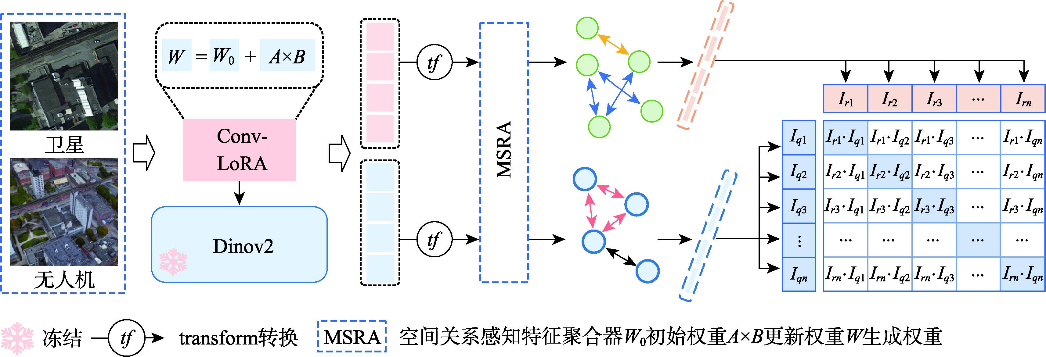
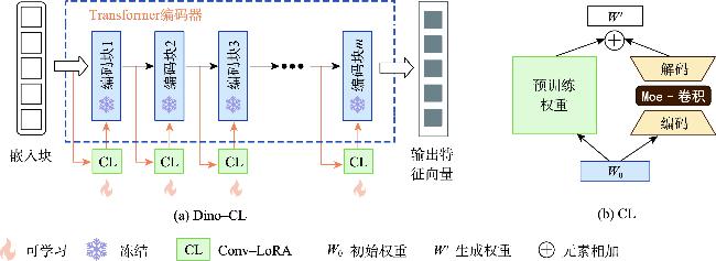
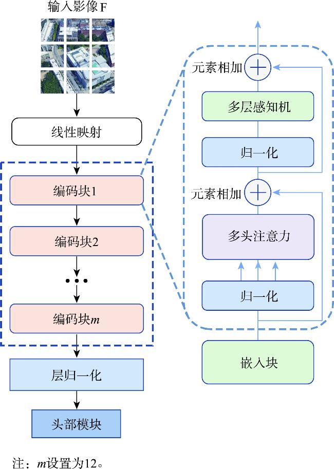
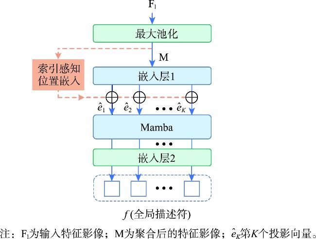
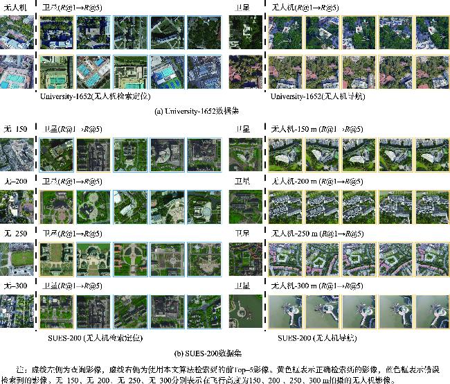
[Objectives] Cross-view image geolocation refers to a technology that determines the geographical location of an image by matching it with reference images taken from different perspectives and possessing precise location information. This technology plays a crucial role in real-world applications such as Unmanned Aerial Vehicle (UAV) navigation, environmental monitoring, and target positioning. Currently, most deep learning-based cross-view image retrieval and geolocation methods for drone-satellite tasks rely heavily on supervised learning. However, the scarcity of high-quality labeled data presents a significant limitation, hindering the generalization capability of these models. Moreover, existing methods often fail to effectively model the spatial layout of images, making it difficult to bridge the substantial domain gap between cross-view images, thereby limiting the accuracy and robustness of geolocation tasks. [Methods] To address these challenges, this paper proposes a novel cross-view image retrieval and localization architecture called DINO-MSRA. The architecture first employs the DINOv2 large model framework, fine-tuned by Conv-LoRA, as the feature encoder. This enhances the model's feature extraction capabilities with fewer parameters, improving both efficiency and accuracy. Second, we design a spatial relation-aware feature aggregator based on the Mamba module (MSRA) to more effectively aggregate image features. By embedding spatial configuration features into the global descriptor, this module significantly improves the model's performance in cross-view matching tasks, especially in complex scenarios where spatial relationships between objects are crucial. Finally, the InfoNCE loss function is adopted to train the model, optimizing contrastive learning and ensuring more accurate retrieval and localization results. [Results] Extensive comparative and ablation experiments were conducted on the University-1652 and SUES-200 datasets. The experimental results show that for drone-view target localization (drone→satellite) and drone navigation (satellite→drone) tasks, the proposed method achieves R@1 accuracies of 95.14% and 97.29%, respectively, on the University-1652 dataset, representing improvements of 0.68% and 1.14% over the current best algorithm, CAMP. On the SUES-200 dataset at an altitude of 150 meters, R@1 accuracies reach 97.2% and 98.75%, which are 1.8% and 2.5% higher than CAMP, respectively. Moreover, the proposed method requires significantly fewer parameters than existing algorithms, only 19.2% of those used by Sample4Geo. [Conclusions] In summary, the proposed DINO-MSRA architecture outperforms current state-of-the-art methods in cross-view image matching, achieving higher accuracy and faster inference speed. These results demonstrate its robustness and practical application potential in challenging real-world scenarios.
PING Yifan , LU Jun , GUO Haitao , HOU Qingfeng , ZHU Kun , SANG Zehao , LIU Tong . DINO-MSRA: A novel Network Architecture for Cross-View Image Retrieval and Localization of UAV and Satellite Images[J]. Journal of Geo-information Science, 2025 , 27(7) : 1608 -1623 . DOI: 10.12082/dqxxkx.2025.250051
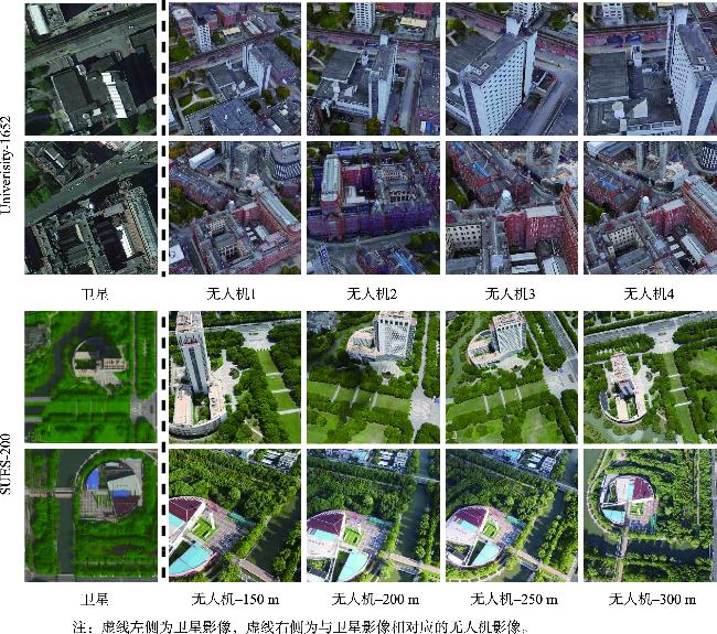
表1 实验数据集详细信息Tab. 1 The detailed information of datasets used in the experiment (张) |
| 数据集 | University-1652 | SUES-200 | ||||
|---|---|---|---|---|---|---|
| 图像数量/张 | 建筑物数量/张 | 图像数量/张 | 建筑物数量/张 | |||
| 训练集 | 卫星 | 701 | 701 | 120 | 120 | |
| 无人机 | 37 854 | 701 | 6 000 | 120 | ||
| 测试集 | 查询无人机 | 37 855 | 701 | 4 000 | 80 | |
| 查询卫星 | 701 | 701 | 200 | 200 | ||
| 卫星影像库 | 951 | 951 | 80 | 80 | ||
| 无人机影像库 | 51 355 | 951 | 10 000 | 200 | ||
注:训练集中的建筑物和测试集中的建筑物没有重叠。 |
表2 各算法在University-1652数据集上的精度对比Tab. 2 Accuracy comparison of various algorithms on the University-1652 dataset |
| 算法 | 输入尺寸 /像素×像素 | 权重共享 | 可学习 参数量/M | 无人机→卫星 | 卫星→无人机 | |||
|---|---|---|---|---|---|---|---|---|
| R@1 | AP | R@1 | AP | |||||
| University-1652[28] | 256×256 | - | - | 58.49 | 63.13 | 71.18 | 58.74 | |
| RK-Net[2] | 256×256 | - | - | 66.13 | 70.23 | 80.17 | 65.76 | |
| LCM[4] | 256×256 | - | - | 66.65 | 70.82 | 79.89 | 65.38 | |
| LPN[32] | 256×256 | × | 138.7×2 | 75.93 | 79.14 | 86.45 | 74.79 | |
| SAIG-D[35] | 256×256 | × | 15.6×2 | 78.85 | 81.62 | 86.45 | 78.48 | |
| DWDR[33] | 256×256 | - | - | 86.41 | 88.41 | 91.30 | 86.02 | |
| MBF[36] | 256×256 | - | - | 89.05 | 90.61 | 92.15 | 84.45 | |
| SeGCN[37] | 256×256 | - | - | 89.18 | 90.89 | 94.29 | 89.65 | |
| Sample4geo[7] | 256×256 | √ | 88.6 | 92.65 | 93.81 | 95.14 | 91.39 | |
| CAMP[6] | 256×256 | - | - | 94.46 | 95.38 | 96.15 | 92.72 | |
| FDER[9] | 256×256 | - | - | 92.79 | 93.91 | 95.58 | 92.17 | |
| FastSAM[11] | 224×224 | - | - | 59.14 | 63.50 | 68.94 | 60.32 | |
| 本文算法 | 224×224 | √ | 17.01 | 95.14 | 95.92 | 97.29 | 93.81 | |
注:加粗数值为每列最优值,“-”表示未知。 |
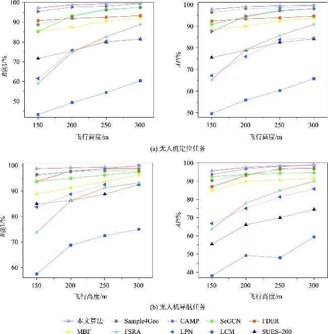
表3 各算法在SUES-200数据集上的精度结果对比(无人机→卫星)Tab. 3 Accuracy comparison of various algorithms on the SUES-200 dataset (Drone → Satellite) |
| 算法 | 输入尺寸 /像素×像素 | 150 m | 200 m | 250 m | 300 m | |||||||
|---|---|---|---|---|---|---|---|---|---|---|---|---|
| R@1 | AP | R@1 | AP | R@1 | AP | R@1 | AP | |||||
| LCM[4] | 256×256 | 43.32 | 49.65 | 49.42 | 55.91 | 54.47 | 60.31 | 60.43 | 65.78 | |||
| LPN[32] | 256×256 | 61.58 | 67.23 | 75.85 | 75.96 | 80.38 | 83.8 | 81.47 | 84.53 | |||
| FSRA[34] | 256×256 | 59.18 | 65.28 | 74.88 | 79.2 | 82.67 | 85.76 | 88.88 | 90.82 | |||
| SUES-200[29] | 256×256 | 71.67 | 75.55 | 75.57 | 78.97 | 79.97 | 82.50 | 81.42 | 84.11 | |||
| MBF[36] | 256×256 | 85.62 | 88.32 | 87.43 | 90.02 | 90.65 | 92.53 | 92.12 | 93.63 | |||
| FDER[9] | 256×256 | 85.30 | 87.58 | 93.23 | 94.66 | 96.47 | 97.28 | 97.50 | 98.09 | |||
| Sample4Geo[7] | 256×256 | 88.77 | 90.89 | 92.8 | 94.29 | 96.22 | 97.03 | 97.44 | 98.02 | |||
| SeGCN[37] | 256×256 | 90.80 | 92.32 | 91.93 | 93.41 | 92.53 | 93.90 | 93.33 | 94.61 | |||
| CAMP[6] | 256×256 | 95.40 | 96.38 | 97.63 | 98.16 | 98.05 | 98.45 | 99.33 | 99.46 | |||
| 本文算法 | 224×224 | 97.2 | 97.82 | 98.75 | 99.03 | 99.38 | 99.47 | 99.63 | 99.71 | |||
注:加粗数值为每列最优值。无人机→卫星表示面向无人机定位任务,其中,无人机影像为查询影像、卫星影像为参考影像。 |
表4 各算法在SUES-200数据集上的精度结果对比(卫星→无人机)Tab. 4 Accuracy comparison of various algorithms on the SUES-200 dataset (Satellite → Drone) |
| 算法 | 输入尺寸 /像素×像素 | 150 m | 200 m | 250 m | 300 m | |||||||
|---|---|---|---|---|---|---|---|---|---|---|---|---|
| R@1 | AP | R@1 | AP | R@1 | AP | R@1 | AP | |||||
| LCM[4] | 256×256 | 57.5 | 38.11 | 68.75 | 49.19 | 72.5 | 47.94 | 75.0 | 59.36 | |||
| LPN[32] | 256×256 | 83.75 | 66.78 | 88.75 | 75.01 | 92.5 | 81.34 | 92.5 | 85.72 | |||
| FSRA[34] | 256×256 | 73.75 | 63.7 | 86.25 | 78.02 | 91.25 | 84.83 | 93.25 | 89.88 | |||
| SUES-200[21] | 256×256 | 85.0 | 71.36 | 86.25 | 75.96 | 88.75 | 79.54 | 92.50 | 84.89 | |||
| MBF[29] | 256×256 | 88.75 | 84.74 | 91.25 | 89.95 | 93.75 | 90.65 | 96.25 | 91.6 | |||
| FDER[9] | 256×256 | 93.75 | 86.93 | 97.75 | 93.12 | 98.75 | 96.81 | 98.75 | 97.20 | |||
| SeGCN[37] | 256×256 | 93.75 | 92.45 | 95.00 | 93.65 | 96.25 | 94.39 | 97.50 | 94.55 | |||
| Sample4Geo[7] | 256×256 | 96.5 | 90.31 | 97.58 | 93.74 | 97.92 | 96.49 | 97.83 | 96.73 | |||
| CAMP[6] | 256×256 | 96.25 | 93.69 | 97.50 | 96.76 | 98.75 | 98.10 | 100 | 98.85 | |||
| 本文算法 | 224×224 | 98.75 | 95.69 | 99.08 | 97.51 | 99.38 | 98.44 | 99.42 | 98.76 | |||
注:加粗数值为每列最优值。卫星→无人机表示面向无人机导航任务,其中,卫星影像为查询影像、无人机影像为参考影像。 |
表5 不同超参数配置在University-1652数据集上的消融实验Tab. 5 Ablation study of different hyperparameter configurations on University-1652 |
| 算法 | 冻结层数 | Conv- LoRA | 可学习参 数量/M | 无人机 → 卫星 | 卫星 → 无人机 | ||||
|---|---|---|---|---|---|---|---|---|---|
| R@1 | AP | R@1 | AP | ||||||
| Dino-MSRA | × | × | 94.40 | 94.58 | 95.43 | 96.15 | 93.02 | ||
| Dino-MSRA | [0-07] | × | 44.77 | 94.64 | 95.51 | 97.15 | 93.41 | ||
| Dino-MSRA | [0-11] | × | 16.42 | 61.71 | 66.56 | 89.73 | 70.69 | ||
| Dino-MSRA | [0-11] | r = 2 | 16.49 | 93.58 | 94.89 | 97.29 | 93.46 | ||
| Dino-MSRA | [0-11] | r = 4 | 16.56 | 94.37 | 95.32 | 97.40 | 93.45 | ||
| Dino-MSRA | [0-11] | r = 8 | 16.71 | 94.70 | 95.60 | 97.43 | 93.90 | ||
| Dino-MSRA | [0-11] | r = 16 | 17.01 | 95.14 | 95.92 | 97.29 | 93.81 | ||
| Dino-MSRA | [0-11] | r = 32 | 17.60 | 94.74 | 95.66 | 96.58 | 93.56 | ||
注:加粗数值为每列最优值;参数Conv-LoRA表示是否使用Conv-LoRA微调策略; ×表示未使用; r表示设置的秩(rank)的大小;可学习参数量表示模型训练过程中实际参与学习的参数量。 |
表6 不同超参数配置在SUES-200数据集上的消融实验(无人机→卫星)Tab. 6 Ablation study of different hyperparameter configurations on SUES-200 (Drone →Satellite) |
| 算法 | 冻结 层数 | Conv- LoRA | 150 m | 200 m | 250 m | 300 m | |||||||
|---|---|---|---|---|---|---|---|---|---|---|---|---|---|
| R@1 | AP | R@1 | AP | R@1 | AP | R@1 | AP | ||||||
| Dino-MSRA | × | × | 96.63 | 97.28 | 97.65 | 98.03 | 98.50 | 98.66 | 99.00 | 99.11 | |||
| Dino-MSRA | [0-07] | × | 97.15 | 97.98 | 98.75 | 98.85 | 99.00 | 99.19 | 99.17 | 99.27 | |||
| Dino-MSRA | [0-11] | × | 69.48 | 73.57 | 73.16 | 79.52 | 78.58 | 84.37 | 85.15 | 87.46 | |||
| Dino-MSRA | [0-11] | r = 2 | 95.83 | 96.67 | 97.56 | 98.15 | 97.58 | 98.26 | 98.60 | 98.83 | |||
| Dino-MSRA | [0-11] | r = 4 | 95.58 | 96.45 | 97.85 | 98.24 | 97.69 | 98.30 | 98.90 | 99.05 | |||
| Dino-MSRA | [0-11] | r = 8 | 96.40 | 97.12 | 97.80 | 98.17 | 97.73 | 98.13 | 98.70 | 98.90 | |||
| Dino-MSRA | [0-11] | r = 16 | 97.20 | 97.82 | 98.70 | 99.03 | 99.38 | 99.47 | 99.63 | 99.71 | |||
| Dino-MSRA | [0-11] | r = 32 | 96.10 | 96.87 | 97.93 | 98.93 | 98.57 | 99.02 | 98.93 | 99.09 | |||
注:加粗数值为每列最优值;参数Conv-LoRA表示是否使用Conv-LoRA微调策略; ×表示未使用; r表示设置的秩的大小;学习参数量表示模型训练过程中实际参与训练的参数量。 |
表7 不同超参数配置在SUES-200数据集上的消融实验(卫星→无人机)Tab. 7 Ablation study of different hyperparameter configurations on SUES-200 (Satellite →Drone) |
| 算法 | 冻结 层数 | Conv- LoRA | 150 m | 200 m | 250 m | 300 m | |||||||
|---|---|---|---|---|---|---|---|---|---|---|---|---|---|
| R@1 | AP | R@1 | AP | R@1 | AP | R@1 | AP | ||||||
| Dino-MSRA | × | × | 97.13 | 95.39 | 97.58 | 96.77 | 98.15 | 97.93 | 98.79 | 98.56 | |||
| Dino-MSRA | [0-07] | × | 98.03 | 95.97 | 98.18 | 97.12 | 98.42 | 98.05 | 98.75 | 98.34 | |||
| Dino-MSRA | [0-11] | × | 90.00 | 65.25 | 93.17 | 80.55 | 96.25 | 92.63 | 97.50 | 84.66 | |||
| Dino-MSRA | [0-11] | r = 2 | 97.90 | 92.48 | 98.14 | 95.36 | 97.72 | 96.90 | 98.75 | 98.01 | |||
| Dino-MSRA | [0-11] | r = 4 | 98.00 | 92.29 | 98.24 | 96.72 | 98.56 | 97.55 | 99.16 | 97.56 | |||
| Dino-MSRA | [0-11] | r = 8 | 98.75 | 94.63 | 99.12 | 97.24 | 99.27 | 97.94 | 99.40 | 98.72 | |||
| Dino-MSRA | [0-11] | r = 16 | 98.75 | 95.69 | 99.08 | 97.51 | 99.38 | 98.44 | 99.42 | 98.76 | |||
| Dino-MSRA | [0-11] | r = 32 | 98.17 | 93.39 | 98.75 | 97.28 | 99.02 | 98.32 | 99.14 | 98.04 | |||
注:加粗数值为每列最优值;参数Conv-LoRA表示是否使用Conv-LoRA微调策略; ×表示未使用; r表示设置的秩的大小;学习参数量表示模型训练过程中实际参与训练的参数量。 |
表8 MSRA聚合策略在Univeristy-1652数据集上的有效性验证Tab. 8 Validation of the effectiveness of the MSRA on Univeristy-1652 dataset |
| 算法 | 无人机→卫星 | 卫星→无人机 | |||
|---|---|---|---|---|---|
| R@1 | AP | R@1 | AP | ||
| Dinov2 GeM | 90.97 | 92.36 | 94.58 | 89.52 | |
| Dinov2 NetVLAD | 92.46 | 93.69 | 95.72 | 92.44 | |
| Dinov2 MixVPR | 94.00 | 95.01 | 96.58 | 92.04 | |
| Dinov2 Geodtr | 95.02 | 95.86 | 97.26 | 93.43 | |
| Dinov2 MSRA | 95.14 | 95.92 | 97.29 | 93.81 | |
注:加粗数值为每列最优值。 |
表9 MSRA聚合策略在SUES-200数据集上的有效性验证(无人机→卫星)Tab. 9 Validation of the effectiveness of the MSRA on SUES-200 dataset (Drone→Satellite) |
| 算法 | 150 m | 200 m | 250 m | 300 m | |||||||
|---|---|---|---|---|---|---|---|---|---|---|---|
| R@1 | AP | R@1 | AP | R@1 | AP | R@1 | AP | ||||
| Dinov2 GeM | 88.43 | 90.64 | 92.70 | 93.15 | 96.05 | 96.58 | 97.28 | 97.74 | |||
| Dinov2 NetVLAD | 92.00 | 93.44 | 95.86 | 96.01 | 97.24 | 97.64 | 99.68 | 99.75 | |||
| Dinov2 MixVPR | 95.05 | 95.98 | 96.15 | 96.98 | 97.09 | 97.78 | 98.80 | 98.99 | |||
| Dinov2 Geodtr | 96.82 | 97.26 | 98.64 | 98.93 | 99.28 | 99.42 | 99.62 | 99.35 | |||
| Dinov2 MSRA | 97.20 | 97.82 | 98.70 | 99.03 | 99.38 | 99.47 | 99.63 | 99.71 | |||
注:加粗数值为每列最优值。 |
表10 MSRA聚合策略在SUES-200数据集上的有效性验证(卫星→无人机)Tab. 10 Validation of the effectiveness of the MSRA on SUES-200 dataset (Satellite→Drone) |
| 算法 | 150 m | 200 m | 250 m | 300 m | |||||||
|---|---|---|---|---|---|---|---|---|---|---|---|
| R@1 | AP | R@1 | AP | R@1 | AP | R@1 | AP | ||||
| Dinov2 GeM | 90.08 | 96.87 | 96.37 | 95.87 | 97.17 | 96.24 | 97.78 | 97.74 | |||
| Dinov2 NetVLAD | 94.13 | 94.7 | 95.93 | 95.23 | 96.05 | 95.98 | 98.75 | 97.46 | |||
| Dinov2 MixVPR | 98.02 | 93.62 | 98.68 | 95.36 | 98.67 | 97.93 | 98.68 | 98.59 | |||
| Dinov2 Geodtr | 98.72 | 95.66 | 98.95 | 97.37 | 99.29 | 98.46 | 99.41 | 98.67 | |||
| Dinov2 MSRA | 98.75 | 95.69 | 99.08 | 97.51 | 99.38 | 98.44 | 99.42 | 98.76 | |||
注:加粗数值为每列最优值。 |
利益冲突:Conflicts of Interest 所有作者声明不存在利益冲突。
All authors disclose no relevant conflicts of interest.
| [1] |
|
| [2] |
|
| [3] |
|
| [4] |
|
| [5] |
|
| [6] |
|
| [7] |
|
| [8] |
|
| [9] |
|
| [10] |
|
| [11] |
|
| [12] |
|
| [13] |
|
| [14] |
|
| [15] |
|
| [16] |
|
| [17] |
|
| [18] |
|
| [19] |
|
| [20] |
|
| [21] |
|
| [22] |
|
| [23] |
|
| [24] |
|
| [25] |
|
| [26] |
|
| [27] |
|
| [28] |
|
| [29] |
|
| [30] |
|
| [31] |
|
| [32] |
|
| [33] |
|
| [34] |
|
| [35] |
|
| [36] |
|
| [37] |
|
/
| 〈 |
|
〉 |