
基于广义回归神经网络的京津冀地区土壤湿度遥感逐日估算研究
|
邓雅文(1999— ),女,湖南衡阳人,硕士生,研究方向为生态水文遥感。E-mail: 202021051199@mail.bnu.edu.cn |
收稿日期: 2020-03-27
要求修回日期: 2020-06-21
网络出版日期: 2021-06-25
基金资助
国家自然科学基金项目(41571077)
国家重点研发计划项目(2016YFC0503002)
环境遥感与数字城市北京 重点实验室开放课题(12800-310430001)
版权
Daily Estimation of Soil Moisture over Beijing-Tianjin-Hebei Region based on General Regression Neural Network Model
Received date: 2020-03-27
Request revised date: 2020-06-21
Online published: 2021-06-25
Supported by
National Natural Science Foundation of China(41571077)
National Key R&D Program of China(2016YFC0503002)
Open subject of Beijing Key Laboratory for Remote Sensing of Environment and Digital Cities(12800-310430001)
Copyright
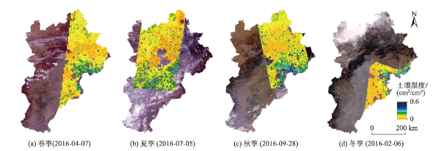
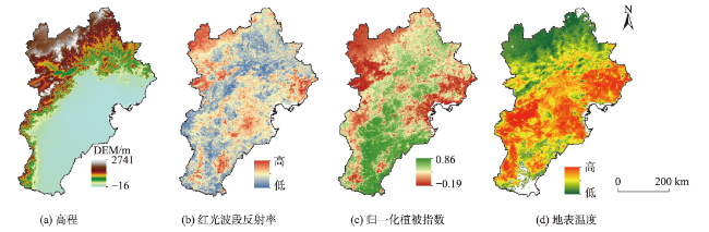
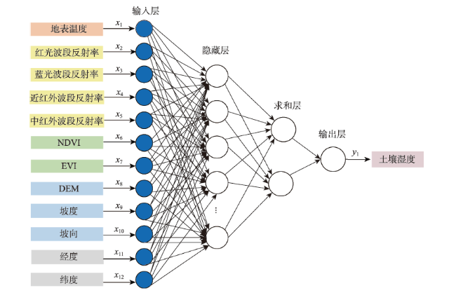
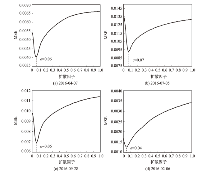
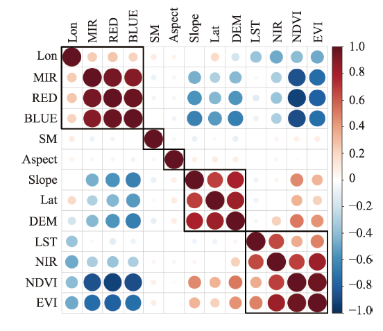
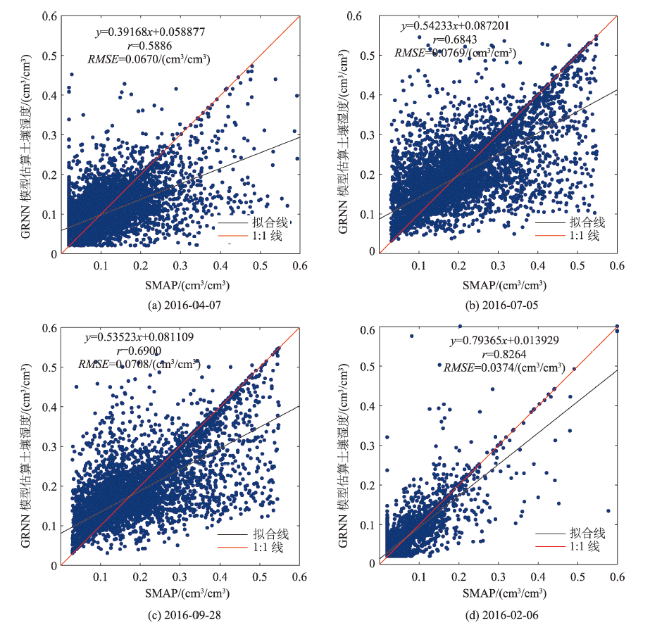
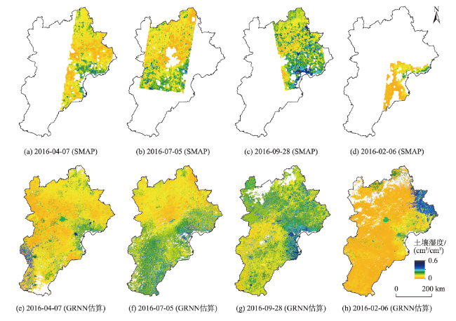
土壤湿度是地表水热交换过程和水文循环中的一个关键组成部分,获取高时空分辨率的土壤湿度数据一直是当前研究的热点。SMAP(Soil Moisture Passive and Active)主被动微波土壤湿度产品的精度高,但存在着空间分辨率低和时间分辨率缺失的问题,这限制了其在区域尺度上的应用,为解决这一问题得到更高时空分辨率的土壤湿度产品,本文利用广义回归神经网络模型(GRNN)模拟了MODIS地表温度、反射率、植被指数光学/热红外遥感数据以及高程、坡度、坡向、经纬度数据与SMAP土壤湿度的关系,从而将京津冀地区SMAP L2土壤湿度产品的时间分辨率由不连续(4~20 d)提升至1 d,空间分辨率由3 km提升至1 km,并扩展其在京津冀地区的空间覆盖范围。研究发现:① GRNN模型总体验证结果表明土壤湿度估算值与SMAP原始值的相关性较高(r=0.7392),均方根误差(RMSE)为0.0757 cm³/cm³;② 不同季节典型日期的GRNN模型估算结果精度相差较大,春季处的相关性相比其他季节最低,精度相对较高(r春=0.6152,RMSE春=0.0653cm³/cm³),秋季和夏季土壤湿度估算精度较为接近(r夏=0.6957,r秋=0.7053,RMSE夏=0.0754cm³/cm³,RMSE秋=0.0694cm³/cm³),冬季的估算精度最高(r冬=0.8214,RMSE冬=0.0367cm³/cm³);③ 2016年京津冀夏秋季节的土壤湿度较其他季节要显著提高,空间分布上坝上高原区域较低,而沿海地区的土壤湿度明显较高。本研究对京津冀地区的生态水文、气候预测以及干旱监测等应用领域具有重要价值。

邓雅文 , 凌子燕 , 孙娜 , 吕金霞 . 基于广义回归神经网络的京津冀地区土壤湿度遥感逐日估算研究[J]. 地球信息科学学报, 2021 , 23(4) : 749 -761 . DOI: 10.12082/dqxxkx.2021.200149
Surface Soil Moisture (SM) plays an important role in the land-atmosphere interaction and hydrological cycle. Low spatiotemporal resolution (i.e., 25~40 km and 2~3 days) microwave-based SM products such as the Soil Moisture and Ocean Salinity (SMOS) and the Advanced Microwave Scanning Radiometer for EOS (AMSR-E) limit their application in regional scale studies. The Soil Moisture Active Passive (SMAP) and Copernicus Sentinel 1A/B microwave active-passive surface soil moisture product (L2_SM_SP) has a higher spatial resolution (3 km), but its temporal resolution is coarse from 4 to 20 days due to the narrow overlapped swath width. In this study, we developed a machine learning algorithm using the General Regression Neural Network (GRNN) to improve the spatiotemporal resolution of the L2_SM_SP product based on multi-source remote sensing data. Land Surface Temperature (LST), Multi-band Reflectance, Normalized Difference Vegetation Index (NDVI), Enhanced Vegetation Index (EVI), Elevation, Slope, Longitude (Lon), and Latitude (Lat) were selected as input variables to simulate the L2_SM_SP soil moisture in GRNN model. Results show that: (1) GRNN-estimated soil moisture and the original estimates of L2_SM_SP were strongly correlated (r=0.7392, RMSE=0.0757 cm3/cm3); (2) the correlation between GRNN estimates and original L2_SM_SP product at typical dates of different seasons varied a lot. The correlation in spring was the lowest (rSpr=0.6152, RMSESpr=0.0653 cm³/cm³). While the correlation in winter was the strongest (rWin=0.8214, and RMSEWin=0.0367 cm3/cm3). The correlation in summer and autumn was close to each other (rSum=0.6957, rAut=0.7053, RMSESum=0.0754 cm³/cm³, and RMSEAut=0.0694 cm³/cm³); and (3) in 2016, the soil moisture in summer and autumn of the study area was significantly higher than that that in other seasons. In terms of spatial distribution, the soil moisture in the Bashang plateau area was low, while the soil moisture along coastal areas was obviously higher. In this study, we successfully improved the spatiotemporal resolution of L2_SM_SP product over Beijing-Tianjin-Hebei region from 3 km, and 4~20 days to 1 km, and 1 day. Its spatial coverage was also extended. The improved soil moisture product is of great significance for future eco-hydrological assessment, climate prediction, and drought monitoring in Beijing-Tianjin-Hebei region.
表1 研究使用的遥感数据列表Tab. 1 Remote sensing data used in this study |
| 数据类型 | 数据名称 | 时间分辨率/d | 空间分辨率 | 产品类型 | 时间节点 | 数据位置 |
|---|---|---|---|---|---|---|
| MODIS | MOD13A2 | 16 | 1 km | 植被指数与反射率 | 2016-04-07 | h26v04, h26v05 |
| MOD11A1 | 1 | 1 km | 地表温度 | 2016-07-05 | h27v04, h27v05 | |
| SMAP | SPL2SMAP_S | 4~20 | 3 km | 土壤湿度 | 2016-09-28 | 116°E—118°E, 37°N—44°N |
| 2016-02-06 | ||||||
| 高程 | DEM | - | 30 m | 高程 | - | - |
表2 对模型输入变量进行主成分分析得到的特征根与方差贡献率Tab. 2 Characteristic roots and variance contribution rates obtained by principal component analysis of model input variables |
| 主成分 | 特征值 | 方差贡献率 | 累计贡献率 |
|---|---|---|---|
| 1 | 5.8544 | 0.488 | 0.488 |
| 2 | 1.8477 | 0.154 | 0.642 |
| 3 | 1.1322 | 0.094 | 0.736 |
| 4 | 0.9806 | 0.082 | 0.818 |
| 5 | 0.7982 | 0.067 | 0.884 |
| 6 | 0.5754 | 0.048 | 0.932 |
| 7 | 0.4060 | 0.034 | 0.966 |
| 8 | 0.2731 | 0.023 | 0.989 |
| 9 | 0.0982 | 0.008 | 0.997 |
| 10 | 0.0257 | 0.002 | 0.999 |
| 11 | 0.0079 | 0.001 | 1.000 |
| 12 | 0.0006 | 0.000 | 1.000 |
表3 GRNN模型输入层变量降维前后的表现对比Tab. 3 Comparison of GRNN model's performance before and after input variables'dimensionality reduction |
| r | RMSE/(cm³/cm³) | bias | ubRMSE | 样本量/个 | 训练时间/s | ||
|---|---|---|---|---|---|---|---|
| GRNN降维前扩散因子为0.09 | 训练精度 | 0.7566 | 0.0736 | -0.0011 | 0.0736 | 48000 | |
| 验证精度 | 0.7322 | 0.0766 | -0.0005 | 0.0765 | 12000 | 1007.75 | |
| 总体精度 | 0.7392 | 0.0757 | -0.0007 | 0.0757 | 60000 | ||
| GRNNPCA降维后扩散因子为0.04 | 训练精度 | 0.7032 | 0.0777 | -0.0002 | 0.0777 | 48000 | |
| 验证精度 | 0.7140 | 0.0787 | 0.0012 | 0.0787 | 12000 | 768.02 | |
| 总体精度 | 0.7110 | 0.0784 | 0.0008 | 0.0784 | 60000 |
表4 不同季节GRNN 1 km土壤湿度的总体评价Tab. 4 Model training accuracy in different seasons |
| 时间 | 指标 | 训练精度 | 验证精度 | 总体精度 | 时间 | 指标 | 训练精度 | 验证精度 | 总体精度 |
|---|---|---|---|---|---|---|---|---|---|
| 春季 (2016-04-07) | r | 0.6300** | 0.5886** | 0.6152** | 秋季 (2016-09-28) | r | 0.7467** | 0.6900** | 0.7053** |
| RMSE/(cm³/cm³) | 0.0636 | 0.0669 | 0.0653 | RMSE/(cm³/cm³) | 0.0658 | 0.0708 | 0.0694 | ||
| bias | 0.0009 | 0.0003 | 0.0005 | bias | 0.0004 | 0.0008 | 0.0007 | ||
| ubRMSE | 0.0636 | 0.0659 | 0.0653 | ubRMSE | 0.0658 | 0.0708 | 0.0694 | ||
| 样本量/个 | 32 000 | 8000 | 40 000 | 样本量/个 | 32 000 | 8000 | 40 000 | ||
| 夏季 (2016-07-05) | r | 0.7277** | 0.6843** | 0.6957** | 冬季 (2016-12-14) | r | 0.8064** | 0.8308** | 0.8214** |
| RMSE/(cm³/cm³) | 0.0715 | 0.0769 | 0.0754 | RMSE/(cm³/cm³) | 0.0348 | 0.0374 | 0.0367 | ||
| bias | 0.0018 | 0.0013 | 0.0014 | bias | -0.0019 | -0.0016 | -0.0017 | ||
| ubRMSE | 0.0715 | 0.0769 | 0.0754 | ubRMSE | 0.0348 | 0.0374 | 0.0367 | ||
| 样本量/个 | 32 000 | 8000 | 40 000 | 样本量/个 | 16 000 | 4000 | 20 000 |
注:**表示通过p<0.01的显著性检验。 |
| [1] |
|
| [2] |
|
| [3] |
|
| [4] |
|
| [5] |
|
| [6] |
丁旭, 赖欣, 范广洲, 等. 中国不同气候区土壤湿度特征及其气候响应[J]. 高原山地气象研究, 2016,36(4):28-35.
[
|
| [7] |
|
| [8] |
|
| [9] |
韩帅, 师春香, 林泓锦, 等. CLDAS土壤湿度业务产品的干旱监测应用[J]. 冰川冻土, 2015,37(2):446-453.
[
|
| [10] |
习阿幸, 刘志辉, 卢文君. 干旱区季节性冻土冻融状况及对融雪径流的影响[J]. 水土保持研究, 2016,23(2):333-339.
[
|
| [11] |
刘荣华, 张珂, 晁丽君, 等. 基于多源卫星观测的中国土壤湿度时空特征分析[J]. 水科学进展, 2017,28(4):479-487.
[
|
| [12] |
孔金玲, 李菁菁, 甄珮珮, 等. 微波与光学遥感协同反演旱区地表土壤湿度研究[J]. 地球信息科学学报, 2016,18(6):857-863.
[
|
| [13] |
陈书林, 刘元波, 温作民. 卫星遥感反演土壤湿度研究综述[J]. 地球科学进展, 2012(11):1192-1203.
[
|
| [14] |
|
| [15] |
|
| [16] |
|
| [17] |
|
| [18] |
|
| [19] |
贾炳浩, 师春香, 孙帅, 等. 基于风云卫星的土壤湿度数据同化研究:第35届中国气象学会年会[ C].中国安徽合肥, 2018.
[
|
| [20] |
|
| [21] |
|
| [22] |
|
| [23] |
贾艳昌, 谢谟文, 姜红涛. 全球36 km格网土壤湿度逐日估算[J]. 地球信息科学学报, 2017,19(6):854-860.
[
|
| [24] |
|
| [25] |
|
| [26] |
|
| [27] |
于占江, 杨鹏. 近50年京津冀气候变化及其对土壤湿度的影响[J]. 贵州农业科学, 2019,47(2):144-149.
[
|
| [28] |
|
| [29] |
李鹏飞, 刘文军, 赵昕奕, 等. 京津冀区域近50年气温、降水与潜在蒸散量变化分析[J]. 干旱区资源与环境, 2015,29(3):137-143.
[
|
| [30] |
张悦, 沈润平, 彭露露, 等. 基于重建MODIS无云数据反演京津冀地区土壤湿度[J]. 江苏农业科学, 2016,44(12):375-378.
[
|
| [31] |
|
| [32] |
|
| [33] |
|
| [34] |
|
/
| 〈 |
|
〉 |